The PANEL Procedure
- Overview
- Getting Started
-
Syntax

-
DetailsSpecifying the Input DataSpecifying the Regression ModelUnbalanced DataMissing ValuesComputational ResourcesRestricted EstimatesNotationOne-Way Fixed-Effects ModelTwo-Way Fixed-Effects ModelBalanced PanelsUnbalanced PanelsFirst-Differenced Methods for One-Way and Two-Way ModelsBetween EstimatorsPooled EstimatorOne-Way Random-Effects ModelTwo-Way Random-Effects ModelParks Method (Autoregressive Model)Da Silva Method (Variance-Component Moving Average Model)Dynamic Panel EstimatorLinear Hypothesis TestingHeteroscedasticity-Corrected Covariance MatricesHeteroscedasticity- and Autocorrelation-Consistent Covariance MatricesR-SquareSpecification TestsPanel Data Poolability TestPanel Data Cross-Sectional Dependence TestPanel Data Unit Root TestsLagrange Multiplier (LM) Tests for Cross-Sectional and Time EffectsTests for Serial Correlation and Cross-Sectional EffectsTroubleshootingCreating ODS GraphicsOUTPUT OUT= Data SetOUTEST= Data SetOUTTRANS= Data SetPrinted OutputODS Table Names
-
Example
- References
Parks (1967) considered the first-order autoregressive model in which the random errors ![]() ,
, ![]() , and
, and ![]() have the structure
have the structure
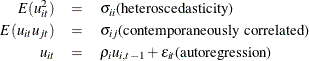
where
The model assumed is first-order autoregressive with contemporaneous correlation between cross sections. In this model, the covariance matrix for the vector of random errors u can be expressed as
![\begin{eqnarray*} {E}( \Strong{uu} ^{'})=\Strong{V} = \left[\begin{matrix} {\sigma }_{11}P_{11} & {\sigma }_{12}P_{12} & {\ldots } & {\sigma }_{1N}P_{1N} \\ {\sigma }_{21}P_{21} & {\sigma }_{22}P_{22} & {\ldots } & {\sigma }_{2N}P_{2N} \\ {\vdots } & {\vdots } & {\vdots } & {\vdots } \\ {\sigma }_{N1}P_{N1} & {\sigma }_{N2}P_{N2} & {\ldots } & {\sigma }_{NN}P_{NN} \\ \end{matrix} \nonumber \right] \end{eqnarray*}](images/etsug_panel0314.png)
where
![\begin{eqnarray*} P_{ij}= \left[\begin{matrix} 1 & {\rho }_{j} & {\rho }_{j}^{2} & {\ldots } & {\rho }^{T-1}_{j} \\ {\rho }_{i} & 1 & {\rho }_{j} & {\ldots } & {\rho }^{T-2}_{j} \\ {\rho }_{i}^{2} & {\rho }_{i} & 1 & {\ldots } & {\rho }^{T-3}_{j} \\ {\vdots } & {\vdots } & {\vdots } & {\vdots } & {\vdots } \\ {\rho }^{T-1}_{i} & {\rho }^{T-2}_{i} & {\rho }^{T-3}_{i} & {\ldots } & 1 \\ \end{matrix} \nonumber \right] \end{eqnarray*}](images/etsug_panel0315.png)
The matrix V is estimated by a two-stage procedure, and ![]() is then estimated by generalized least squares. The first step in estimating V involves the use of ordinary least squares to estimate
is then estimated by generalized least squares. The first step in estimating V involves the use of ordinary least squares to estimate ![]() and obtain the fitted residuals, as follows:
and obtain the fitted residuals, as follows:
A consistent estimator of the first-order autoregressive parameter is then obtained in the usual manner, as follows:
Finally, the autoregressive characteristic of the data is removed (asymptotically) by the usual transformation of taking
weighted differences. That is, for ![]() ,
,
which is written
Notice that the transformed model has not lost any observations (Seely and Zyskind, 1971).
The second step in estimating the covariance matrix V is applying ordinary least squares to the preceding transformed model, obtaining
from which the consistent estimator of ![]()
![]() is calculated as follows:
is calculated as follows:
where
Estimated generalized least squares (EGLS) then proceeds in the usual manner,
where ![]() is the derived consistent estimator of V. For computational purposes,
is the derived consistent estimator of V. For computational purposes, ![]() is obtained directly from the transformed model,
is obtained directly from the transformed model,
where ![]() .
.
The preceding procedure is equivalent to Zellner’s two-stage methodology applied to the transformed model (Zellner, 1962).
Parks demonstrates that this estimator is consistent and asymptotically, normally distributed with
For the PARKS option, the first-order autocorrelation coefficient must be estimated for each cross section. Let ![]() be the
be the ![]() vector of true parameters and
vector of true parameters and ![]() be the corresponding vector of estimates. Then, to ensure that only range-preserving estimates are used in PROC PANEL, the
following modification for R is made:
be the corresponding vector of estimates. Then, to ensure that only range-preserving estimates are used in PROC PANEL, the
following modification for R is made:
![\[ r_{i} = \begin{cases} r_{i} & \mr{if} \hspace{.1 in}{|r_{i}|}<1 \\ \mr{max}(.95, \mr{rmax}) & \mr{if}\hspace{.1 in} r_{i}{\ge }1 \\ \mr{min}(-.95, \mr{rmin}) & \mr{if}\hspace{.1 in} r_{i}{\le }-1 \end{cases} \]](images/etsug_panel0337.png)
where
and
Whenever this correction is made, a warning message is printed.