The PANEL Procedure
- Overview
- Getting Started
-
Syntax

-
DetailsSpecifying the Input DataSpecifying the Regression ModelUnbalanced DataMissing ValuesComputational ResourcesRestricted EstimatesNotationOne-Way Fixed-Effects ModelTwo-Way Fixed-Effects ModelBalanced PanelsUnbalanced PanelsFirst-Differenced Methods for One-Way and Two-Way ModelsBetween EstimatorsPooled EstimatorOne-Way Random-Effects ModelTwo-Way Random-Effects ModelParks Method (Autoregressive Model)Da Silva Method (Variance-Component Moving Average Model)Dynamic Panel EstimatorLinear Hypothesis TestingHeteroscedasticity-Corrected Covariance MatricesHeteroscedasticity- and Autocorrelation-Consistent Covariance MatricesR-SquareSpecification TestsPanel Data Poolability TestPanel Data Cross-Sectional Dependence TestPanel Data Unit Root TestsLagrange Multiplier (LM) Tests for Cross-Sectional and Time EffectsTests for Serial Correlation and Cross-Sectional EffectsTroubleshootingCreating ODS GraphicsOUTPUT OUT= Data SetOUTEST= Data SetOUTTRANS= Data SetPrinted OutputODS Table Names
-
Example
- References
The specification for the two-way random-effects model is
As in the one-way random-effects model, the PANEL procedure provides four options for variance component estimators. Unlike the one-way random-effects model, unbalanced panels present some special concerns.
Let ![]() and
and ![]() be the independent and dependent variables arranged by time and by cross section within each time period. (Note that the
input data set used by the PANEL procedure must be sorted by cross section and then by time within each cross section.) Let
be the independent and dependent variables arranged by time and by cross section within each time period. (Note that the
input data set used by the PANEL procedure must be sorted by cross section and then by time within each cross section.) Let
![]() be the number of cross sections observed in time
be the number of cross sections observed in time ![]() and
and ![]() . Let
. Let ![]() be the
be the ![]() matrix obtained from the
matrix obtained from the ![]() identity matrix from which rows that correspond to cross sections not observed at time
identity matrix from which rows that correspond to cross sections not observed at time ![]() have been omitted. Consider
have been omitted. Consider
where ![]() and
and ![]() .
.
The matrix ![]() gives the dummy variable structure for the two-way model.
gives the dummy variable structure for the two-way model.
For notational ease, let
The Fuller and Battese method for estimating variance components can be obtained by setting VCOMP = FB (with the option RANTWO). FB is the default method for a RANTWO model with balanced panel. If RANTWO is requested without specifying the VCOMP= option, PROC PANEL proceeds under the Fuller and Battese method.
Following the discussion in Baltagi, Song, and Jung (2002), the Fuller and Battese method forms the estimates as follows.
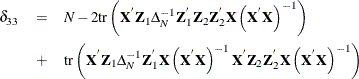
The estimator of the error variance is
where ![]() is the Wansbeek and Kapteyn within estimator for unbalanced (or balanced) panel in a two-way setting.
is the Wansbeek and Kapteyn within estimator for unbalanced (or balanced) panel in a two-way setting.
The estimator of the error variance is the same as that in the Wansbeek and Kapteyn method.
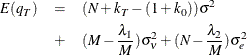
Consider the expected values
![\begin{eqnarray*} \emph{E} (q_{N}) & =& {\sigma }^{2}_{{\epsilon }}\left[M - T - K + 1 \right] \\ & +& {\sigma }^{2}_{{\nu }}\left[ M - T - \mr{tr}\left(\Strong{X}_{s}^{'}{\bar{\Delta }}_{2}\Strong{Z}_{1}\Strong{Z}_{1}^{'}{\bar{\Delta }}_{2}\Strong{X}_{s} \left(\Strong{X}_{s}^{'}{\bar{\Delta }}_{2}\Strong{X}_{s}\right)^{-1}\right)\right]\\ \emph{E} (q_{T}) & =& {\sigma }^{2}_{{\epsilon }}\left[M - N - K + 1 \right] \\ & +& {\sigma }^{2}_{e}\left[ M - N - \mr{tr}\left(\Strong{X}_{s}^{'}{\bar{\Delta }}_{1}\Strong{Z}_{2}\Strong{Z}_{2}^{'}{\bar{\Delta }}_{1}\Strong{X}_{s} \left(\Strong{X}_{s}^{'}{\bar{\Delta }}_{1}\Strong{X}_{s}\right)^{-1}\right)\right] \end{eqnarray*}](images/etsug_panel0255.png)
Just as in the one-way case, there is always the possibility that the (estimated) variance components will be negative. In
such a case, the negative components are fixed to equal zero. After substituting the group sum of the within residuals for
![]() , the time sums of the within residuals for
, the time sums of the within residuals for ![]() , and
, and ![]() , the two equations are solved for
, the two equations are solved for ![]() and
and ![]() .
.
The Wansbeek and Kapteyn method for estimating variance components can be obtained by setting VCOMP = WK. The following methodology, outlined in Wansbeek and Kapteyn (1989) is used to handle both balanced and unbalanced data. The Wansbeek and Kapteyn method is the default for a RANTWO model with unbalanced panel. If RANTWO is requested without specifying the VCOMP= option, PROC PANEL proceeds under the Wansbeek and Kapteyn method if the panel is unbalanced.
The estimator of the error variance is
where the ![]() are given by
are given by ![]() if there is an intercept and by
if there is an intercept and by ![]() if there is not.
if there is not.
The estimation of the variance components is performed by using a quadratic unbiased estimation (QUE) method that involves
computing on quadratic forms of the residuals ![]() , equating their expected values to the realized quadratic forms, and solving for the variance components.
, equating their expected values to the realized quadratic forms, and solving for the variance components.
Let
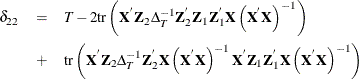
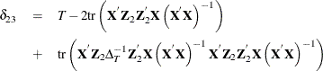
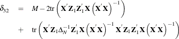
The expected values are
where
The quadratic unbiased estimators for ![]() and
and ![]() are obtained by equating the expected values to the quadratic forms and solving for the two unknowns.
are obtained by equating the expected values to the quadratic forms and solving for the two unknowns.
When the NOINT option is specified, the variance component equations change slightly. In particular, the following is true (Wansbeek and Kapteyn, 1989):
The Wallace and Hussain method for estimating variance components can be obtained by setting VCOMP = WH. Wallace and Hussain’s method is by far the most computationally intensive. It uses the OLS residuals to estimate the variance components. In other words, the Wallace and Hussain method assumes that the following holds:
Taking expectations yields
where the ![]() constants are defined by
constants are defined by
The PANEL procedure solves this system for the estimates ![]() ,
, ![]() , and
, and ![]() . Some of the estimated variance components can be negative. Negative components are set to zero and estimation proceeds.
. Some of the estimated variance components can be negative. Negative components are set to zero and estimation proceeds.
The Nerlove method for estimating variance components can be obtained with by setting VCOMP = NL.
The estimator of the error variance is
The variance components for cross section and time effects are:
and
After you calculate the estimates of the variance components, you can proceed to the final estimation. If the panel is balanced, partial mean deviations are used:
The ![]() estimates are obtained from:
estimates are obtained from:
With these partial deviations, PROC PANEL uses OLS on the transformed series (including an intercept if you want).
The case of an unbalanced panel is somewhat more complicated. You could naively substitute the variance components in the equation below:
After inverting the expression for ![]() , it is possible to do GLS on the data (even if the panel is unbalanced). However, the inversion of
, it is possible to do GLS on the data (even if the panel is unbalanced). However, the inversion of ![]() is no small matter because the dimension is at least
is no small matter because the dimension is at least ![]() .
.
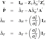
Wansbeek and Kapteyn show that the inverse of ![]() can be written as
can be written as
with the following:
Computationally, this is a much less intensive approach.
By using the inverse of the covariance matrix of the error, it becomes possible to complete GLS on the unbalanced panel.