The PANEL Procedure
- Overview
- Getting Started
-
Syntax

-
DetailsSpecifying the Input DataSpecifying the Regression ModelUnbalanced DataMissing ValuesComputational ResourcesRestricted EstimatesNotationOne-Way Fixed-Effects ModelTwo-Way Fixed-Effects ModelBalanced PanelsUnbalanced PanelsFirst-Differenced Methods for One-Way and Two-Way ModelsBetween EstimatorsPooled EstimatorOne-Way Random-Effects ModelTwo-Way Random-Effects ModelParks Method (Autoregressive Model)Da Silva Method (Variance-Component Moving Average Model)Dynamic Panel EstimatorLinear Hypothesis TestingHeteroscedasticity-Corrected Covariance MatricesHeteroscedasticity- and Autocorrelation-Consistent Covariance MatricesR-SquareSpecification TestsPanel Data Poolability TestPanel Data Cross-Sectional Dependence TestPanel Data Unit Root TestsLagrange Multiplier (LM) Tests for Cross-Sectional and Time EffectsTests for Serial Correlation and Cross-Sectional EffectsTroubleshootingCreating ODS GraphicsOUTPUT OUT= Data SetOUTEST= Data SetOUTTRANS= Data SetPrinted OutputODS Table Names
-
Example
- References
Let ![]() and
and ![]() be the independent and dependent variables arranged by time and by cross section within each time period. (Note that the
input data set used by the PANEL procedure must be sorted by cross section and then by time within each cross section.) Let
be the independent and dependent variables arranged by time and by cross section within each time period. (Note that the
input data set used by the PANEL procedure must be sorted by cross section and then by time within each cross section.) Let
![]() be the number of cross sections observed in year
be the number of cross sections observed in year ![]() and let
and let ![]() . Let
. Let ![]() be the
be the ![]() matrix obtained from the
matrix obtained from the ![]() identity matrix from which rows that correspond to cross sections not observed at time
identity matrix from which rows that correspond to cross sections not observed at time ![]() have been omitted. Consider
have been omitted. Consider
where ![]() and
and ![]() . The matrix
. The matrix ![]() gives the dummy variable structure for the two-way model.
gives the dummy variable structure for the two-way model.
Let
The estimate of the regression slope coefficients is given by
where ![]() is the
is the ![]() matrix without the vector of 1s.
matrix without the vector of 1s.
The estimator of the error variance is
where the residuals are given by ![]() if there is an intercept in the model and by
if there is an intercept in the model and by ![]() if there is no intercept.
if there is no intercept.
The actual implementation is quite different from the theory. The PANEL procedure transforms all series using the ![]() matrix.
matrix.
The variable being transformed is ![]() , which could be
, which could be ![]() or any column of
or any column of ![]() . After the data are properly transformed, OLS is run on the resulting series.
. After the data are properly transformed, OLS is run on the resulting series.
Given ![]() , the next step is estimating the cross-sectional and time effects. Given that
, the next step is estimating the cross-sectional and time effects. Given that ![]() is the column vector of cross-sectional effects and
is the column vector of cross-sectional effects and ![]() is the column vector of time effects,
is the column vector of time effects,
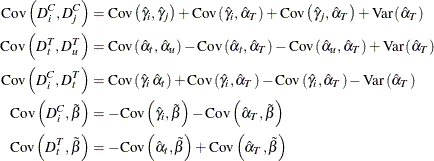
Given the cross-sectional and time effects, the next step is to derive the associated dummy variables. Using the NOINT option, the following equations give the dummy variables:
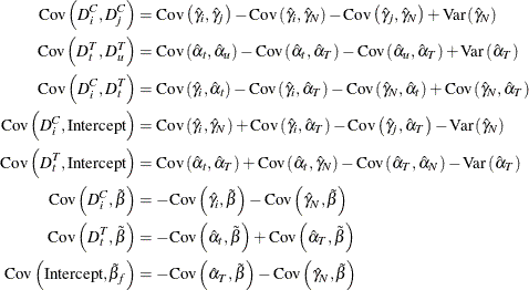
When an intercept is desired, the equations for dummy variables and intercept are:
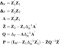
The calculation of the covariance matrix is as follows:
![\begin{eqnarray*} \mr{Var}\left[\hat{\bgamma } \right] & =& \hat{\sigma }_{\epsilon }^{2}\left( \Delta _\emph {N} ^{-1}- {\Sigma }_{1} + {\Sigma }_{2} \right) \\ & +& (\Theta _{1} + \Theta _{2}- \Theta _{3}) \mr{Var}\left[{\tilde{\beta }}_{s}\right] (\Theta _{1} + \Theta _{2}- \Theta _{3})^{'} \end{eqnarray*}](images/etsug_panel0161.png)
where
![\begin{eqnarray*} \mr{Cov}\left[\hat{\balpha }, \hat{\bgamma }^{'}\right] & =& \hat{\sigma }_{\epsilon }^{2}{\Delta }_{N}^{-1} \left[\Strong{A} ^{'}\Strong{Q} ^{-1}{\Delta }_{T}- \Strong{A} ^{'}\Strong{Q} ^{-1}\Strong{A} {\Delta }_{N}^{-1}\Strong{A} ^{'}\right]\Strong{Q} ^{-1} \\ & +& (\Theta _{1} + \Theta _{2}- \Theta _{3}) \mr{Var}\left[{\tilde{\beta }}_{s}\right] \left(\Strong{X} _\mi {s} ^{'}\bar{\mb{Z}} \mb{Q} ^{-1}\right) \end{eqnarray*}](images/etsug_panel0165.png)
Now you work out the variance covariance estimates for the dummy variables.
The variances and covariances of the dummy variables are given under the NOINT selection as follows: