The GAMPL Procedure
-
Overview

- Getting Started
-
Syntax
-
DetailsMissing ValuesThin-Plate Regression SplinesGeneralized Additive ModelsModel Evaluation CriteriaFitting AlgorithmsDegrees of FreedomModel InferenceDispersion ParameterTests for Smoothing ComponentsComputational Method: MultithreadingChoosing an Optimization TechniqueDisplayed OutputODS Table NamesODS Graphics
-
Examples
- References
Getting Started: GAMPL Procedure
This example concerns the proportions and demographic and geographic characteristics of votes that were cast in 3,107 counties
in the United States in the 1980 presidential election. You can use the data set sashelp.Vote1980 directly from the SASHELP library or download it from the StatLib Datasets Archive (Vlachos 1998). For more information about the data set, see Pace and Barry (1997).
The data set contains 3,107 observations and seven variables. The dependent variable LogVoteRate is the logarithm transformation of the proportion of the county population who voted for any candidate. The six explanatory
variables are the number of people in the county 18 years of age or older (Pop), the number of people in the county who have a 12th-grade or higher education (Edu), the number of owned housing units (Houses), the aggregate income (Income), and the scaled longitude and latitude of geographic centroids (Longitude and Latitude).
The following statements produce the plot of LogVoteRate with respect to the geographic locations Longitude and Latitude:
%let off0 = offsetmin=0 offsetmax=0
            linearopts=(thresholdmin=0 thresholdmax=0);
proc template;
   define statgraph surface;
      dynamic _title _z;
      begingraph / designwidth=defaultDesignHeight;
         entrytitle _title;
         layout overlay / xaxisopts=(&off0) yaxisopts=(&off0);
            contourplotparm z=_z y=Latitude x=Longitude / gridded=FALSE;
         endlayout;
      endgraph;
   end;
run;

proc sgrender data=sashelp.Vote1980 template=surface;
   dynamic _title = 'US County Vote Proportion in the 1980 Election'
          _z      = 'LogVoteRate';
run;
Figure 42.1 shows the map of the logarithm transformation of the proportion of the county population who voted for any candidate in the 1980 US presidential election.
Figure 42.1: US County Vote Proportion in the 1980 Election
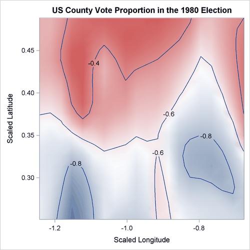
The objective is to explore the nonlinear dependency structure between the dependent variable and demographic variables (Pop, Edu, Houses, and Income), in addition to the spatial variations on geographic variables (Longitude and Latitude). The following statements use thin-plate regression splines to fit a generalized additive model:
ods graphics on;

proc gampl data=sashelp.Vote1980 plots seed=12345;
   model LogVoteRate = spline(Pop   ) spline(Edu) spline(Houses)
                       spline(Income) spline(Longitude Latitude);
   id Longitude Latitude;
   output out=VotePred;
run;
With ODS Graphics enabled by the first statement, the PLOTS option in the PROC GAMPL statement requests a smoothing component panel of fitted spline terms. The SEED option specifies the random seed so that you can reproduce the analysis.
The default output from this analysis is presented in Figure 42.2 through Figure 42.10.
The “Performance Information” table in Figure 42.2 shows that PROC GAMPL executed in single-machine mode (that is, on the server where SAS is installed). When high-performance procedures run in single-machine mode, they use concurrently scheduled threads. In this case, four threads were used.
Figure 42.2: Performance Information
Figure 42.3 displays the “Model Information” table. The response variable LogVoteRate is modeled by using a normal distribution whose mean is modeled by an identity link function. The GAMPL procedure uses the
performance iteration method and the GCV criterion as the fitting criterion. PROC GAMPL searches for the optimum smoothing
parameters by using the Newton-Raphson algorithm to optimize the fitting criterion. The random number seed is set to 12,345.
Random number generation is used for sampling from observations to form spline knots and truncated eigendecomposition. Changing
the random number seed might yield slightly different model fits.
Figure 42.3: Model Information
Figure 42.4 displays the “Number of Observations” table. All 3,107 observations in the data set are used in the analysis. For data sets that have missing or invalid values, the number of used observations might be less than the number of observations read.
Figure 42.4: Number of Observations
Figure 42.5 displays the convergence status of the performance iteration method.
Figure 42.6 shows the “Fit Statistics” table. The penalized log likelihood and the roughness penalty are displayed. You can use effective degrees of freedom to compare generalized additive models with generalized linear models that do not have spline transformations. Information criteria such as Akaike’s information criterion (AIC), Akaike’s bias-corrected information criterion (AICC), and Schwarz Bayesian information criterion (BIC) can also be used for comparisons. These criteria penalize the –2 log likelihood for effective degrees of freedom. The GCV criterion is used to compare against other generalized additive models or models that are penalized.
Figure 42.6: Fit Statistics
| Fit Statistics | |
|---|---|
| Penalized Log Likelihood | 2729.51482 |
| Roughness Penalty | 0.25787 |
| Effective Degrees of Freedom | 48.70944 |
| Effective Degrees of Freedom for Error | 3055.44725 |
| AIC (smaller is better) | -5361.86863 |
| AICC (smaller is better) | -5360.28467 |
| BIC (smaller is better) | -5067.59479 |
| GCV (smaller is better) | 0.01042 |
.
The “Parameter Estimates” table in Figure 42.7 shows the regression parameter and dispersion parameter estimates. In this model, the intercept is the only regression parameter because (1) all variables are characterized by spline terms and no parametric effects are present and (2) the intercept absorbs the constant effect that is extracted from each spline term to make fitted splines identifiable. The dispersion parameter is estimated by maximizing the likelihood, given other model parameters.
Figure 42.7: Regression Parameter Estimates
The “Estimates for Smoothing Components” table is shown in Figure 42.8. For each spline term, the effective degrees of freedom, the estimated smoothing parameter, and the corresponding roughness penalty are displayed. The table also displays additional information about spline terms, such as the number of parameters, penalty matrix rank, and number of spline knots.
Figure 42.8: Estimates for Smoothing Components
| Estimates for Smoothing Components | ||||||
|---|---|---|---|---|---|---|
| Component | Effective DF |
Smoothing Parameter |
Roughness Penalty |
Number of Parameters |
Rank of Penalty Matrix |
Number of Knots |
| Spline(Pop) | 7.80559 | 0.0398 | 0.0114 | 9 | 10 | 2000 |
| Spline(Edu) | 7.12453 | 0.2729 | 0.0303 | 9 | 10 | 2000 |
| Spline(Houses) | 7.20940 | 0.1771 | 0.0370 | 9 | 10 | 2000 |
| Spline(Income) | 5.92854 | 0.7498 | 0.0488 | 9 | 10 | 2000 |
| Spline(Longitude Latitude) | 18.64138 | 0.000359 | 0.1304 | 19 | 20 | 2000 |
Figure 42.9 displays the hypothesis testing results for each smoothing component. The null hypothesis for each spline term is whether the total dependency on each variable is 0. The effective degrees of freedom for both fit and test is displayed.
Figure 42.9: Tests for Smoothing Components
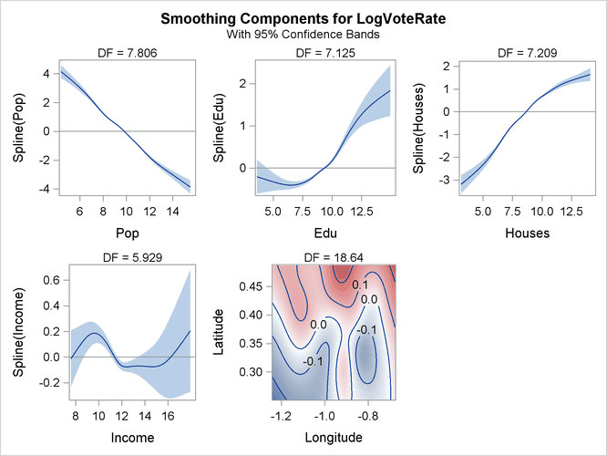
Figure 42.10 displays the “Smoothing Component Panel” for all the spline terms used in the model. It displays predicted spline curves and 95% Bayesian posterior confidence bands for each univariate spline term.
Figure 42.10: Smoothing Component Panel
The preceding program contains an ID statement and an OUTPUT statement. The ID statement transfers the specified variables
(Longitude and Latitude) from the input data set, sashelp.Vote1980, to the output data set, VotePred. The OUTPUT statement requests the prediction for each observation by default and saves the results in the data set VotePred. The following run of the SGRENDER procedure produces the fitted surface of the log vote proportion in the 1980 presidential
election:
proc sgrender data=VotePred template=surface;
   dynamic _title='Predicted US County Vote Proportion in the 1980 Election'
           _z    ='Pred';
run;
Figure 42.11 shows the map of predictions of the logarithm transformation of the proportion of county population who voted for any candidates in the 1980 US presidential election from the fitted generalized additive model.
Figure 42.11: Predicted US County Vote Proportion in the 1980 Election
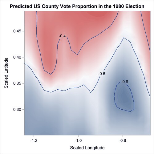
Compared to the map of the logarithm transformations of the proportion of votes cast shown in Figure 42.1, the map of the predictions of the logarithm transformations of the proportion of votes cast has a smoother surface.