The GAMPL Procedure
-
Overview

- Getting Started
-
Syntax
-
DetailsMissing ValuesThin-Plate Regression SplinesGeneralized Additive ModelsModel Evaluation CriteriaFitting AlgorithmsDegrees of FreedomModel InferenceDispersion ParameterTests for Smoothing ComponentsComputational Method: MultithreadingChoosing an Optimization TechniqueDisplayed OutputODS Table NamesODS Graphics
-
Examples
- References
Fitting Algorithms
For models that assume a normally distributed response variable, you can minimize the model evaluation criteria directly by searching for optimal smoothing parameters. For models that have nonnormal distributions, you cannot use the model evaluation criteria directly because the involved statistics keep changing between iterations. The GAMPL procedure enables you to use either of two fitting approaches to search for optimum models: the outer iteration method and the performance iteration method. The outer iteration method modifies the model evaluation criteria so that a global objective function can be minimized in order to find the best smoothing parameters. The performance iteration method minimizes a series of objective functions in an iterative fashion and then obtains the optimum smoothing parameters at convergence. For large data sets, the performance iteration method usually converges faster than the outer iteration method.
Outer Iteration
The outer iteration method is outlined in Wood (2006). The method uses modified model evaluation criteria, which are defined as follows:
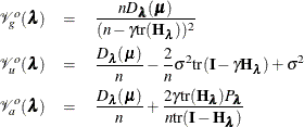
By replacing  with model deviance
  , the modified model evaluation criteria relate to the smoothing parameter
  in a direct way such that the analytic gradient and Hessian are available in explicit forms. The Pearson’s statistic
  is used in the GACV criterion
  (Wood 2008). The algorithm for the outer iteration is thus as follows:
-
Initialize smoothing parameters by taking one step of performance iteration based on adjusted response and adjusted weight except for spline terms with initial values that are specified in the INITSMOOTH= option.
-
Search for the best smoothing parameters by minimizing the modified model evaluation criteria. The optimization process stops when any of the convergence criteria that are specified in the SMOOTHOPTIONS option is met. At each optimization step:
-
Initialize by setting initial regression parameters
 . Set the initial dispersion parameter if necessary.
-
Search for the best regression parameters
 by minimizing the penalized deviance
  (or maximizing the penalized likelihood
  for negative binomial distribution). The optimization process stops when any of the convergence criteria that are specified
in the PLIKEOPTIONS
option is met.
for negative binomial distribution). The optimization process stops when any of the convergence criteria that are specified
in the PLIKEOPTIONS
option is met.
-
At convergence, evaluate derivatives of the model evaluation criteria with respect to
by using  ,
,  ,
,  , and
, and  .
.
-
Step 2b usually converges quickly because it is essentially penalized likelihood estimation given that  . Step 2c contains involved computation by using the chain rule of derivatives. For more information about computing derivatives
of
. Step 2c contains involved computation by using the chain rule of derivatives. For more information about computing derivatives
of  and
and  , see Wood (2008, 2011).
Performance Iteration
The performance iteration method is proposed by Gu and Wahba (1991). Wood (2004) modifies and stabilizes the algorithm for fitting generalized additive models. The algorithm for the performance iteration method is as follows:
-
Initialize smoothing parameters
 , except for spline terms whose initial values are specified in the INITSMOOTH=
option. Set the initial regression parameters
, except for spline terms whose initial values are specified in the INITSMOOTH=
option. Set the initial regression parameters  . Set the initial dispersion parameter if necessary.
-
Repeat the following steps until any of these three conditions is met: (1) the absolute function change in penalized likelihood is sufficiently small; (2) the absolute relative function change in penalized likelihood is sufficiently small; (3) the number of iterations exceeds the maximum iteration limit .
-
Form the adjusted response and adjusted weight from
 . For each observation,
![\[ z_ i=\eta _ i+(y_ i-\mu _ i)/\mu _ i’, \quad w_ i=\omega _ i\mu _ i’^2/\nu _ i \]](images/statug_hpgam0180.png)
-
Search for the best smoothing parameters for the current iteration based on valid adjusted response values and adjusted weight values.
-
Use the smoothing parameters to construct the linear predictor and the predicted means.
-
Obtain an estimate for the dispersion parameter if necessary.
-
In step 2b, you can use different optimization techniques to search for the best smoothing parameters. The Newton-Raphson
optimization is efficient in finding the optimum where the first- and second-order derivatives are available. For more information about computing derivatives of  and
and  with respect to , see Wood (2004).