The GAMPL Procedure
-
Overview

- Getting Started
-
Syntax
-
DetailsMissing ValuesThin-Plate Regression SplinesGeneralized Additive ModelsModel Evaluation CriteriaFitting AlgorithmsDegrees of FreedomModel InferenceDispersion ParameterTests for Smoothing ComponentsComputational Method: MultithreadingChoosing an Optimization TechniqueDisplayed OutputODS Table NamesODS Graphics
-
Examples
- References
Example 42.3 Nonparametric Negative Binomial Model for Mackerel Egg Density
This example demonstrates how you can use PROC GAMPL to fit a nonparametric negative binomial model for a count data set that has overdispersions.
The example concerns a study of mackerel egg density. The data are a subset of the 1992 mackerel egg survey that was conducted over the Porcupine Bank west of Ireland. The survey took place in the peak spawning area. Scientists took samples by hauling a net up from deep sea to the sea surface. Then they counted the number of spawned mackerel eggs and used other geographic information to estimate the sizes and distributions of spawning stocks. The data set is used as an example in Bowman and Azzalini (1997).
The following DATA step creates the data set Mackerel. This data set contains 634 observations and five variables. The response variable Egg_Count is the number of mackerel eggs that are collected from each sampling net. Longitude and Latitude are the location values in degrees east and north, respectively, of each sample station. Net_Area is the area of the sampling net in square meters. Depth records the sea bed depth in meters at the sampling location, and Distance is the distance in geographic degrees from the sample location to the continental shelf edge.
title 'Mackerel Egg Density Study';
data Mackerel;
   input Egg_Count Longitude Latitude  Net_Area Depth Distance;
   datalines;
   0     -4.65     44.57     0.242    4342    0.8395141177
   0     -4.48     44.57     0.242    4334    0.8591926336
   0      -4.3     44.57     0.242    4286    0.8930152895
   1     -2.87     44.02     0.242    1438    0.3956408691
   4     -2.07     44.02     0.242     166    0.0400088237
   3     -2.13     44.02     0.242     460    0.0974234463
   0     -2.27     44.02     0.242     810    0.2362566569

   ... more lines ...

  22     -4.22     46.25      0.19     205    0.1181120828
  21     -4.28     46.25      0.19     237     0.129990854
   0     -4.73     46.25      0.19    2500    0.3346500536
   5     -4.25     47.23      0.19     114     0.718192582
   3     -3.72     47.25      0.19     100    0.9944669778
   0     -3.25     47.25      0.19      64    1.2639918431
;
The response values are counts, so the Poisson distribution might be a reasonable model. The statistic of interest is the mackerel egg density, which can be formed as
![\[ \mathrm{Density} = E(\mathrm{Count})/\mathrm{Net\_ Area} \]](images/statug_hpgam0244.png)
This is equivalent to a Poisson regression that uses the response variable Egg_Count, an offset variable  , and other covariates.
The following statements produce the plot of the mackerel egg density with respect to the sampling station location:
data Temp;
   set Mackerel;
   Density = Egg_Count/Net_Area;
run;
%let off0 = offsetmin=0 offsetmax=0
            linearopts=(thresholdmin=0 thresholdmax=0);
%let off0 = xaxisopts=(&off0) yaxisopts=(&off0);
proc template;
   define statgraph surface;
      dynamic _title _z;
      begingraph / designwidth=defaultDesignHeight;
         entrytitle _title;
         layout overlay / &off0;
            contourplotparm z=_z y=Latitude x=Longitude / gridded=FALSE;
         endlayout;
      endgraph;
   end;
run;

proc sgrender data=Temp template=surface;
   dynamic _title='Mackerel Egg Density' _z='Density';
run;
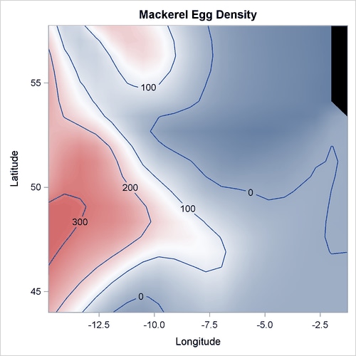
Output 42.3.1 displays the mackerel egg density in the sampling area. The black hole in the upper right corner is caused by missing values in that area.
Output 42.3.1: Mackerel Egg Density
In this example, the dependent variable is the mackerel egg count, the independent variables are the geographical information
about each of the sampling stations, and the offset variable is the logarithm of the sampling area. The following statements
use PROC GAMPL to fit the nonparametric Poisson regression model. In the program, two univariate spline terms for Depth and Distance model the nonlinear dependency of egg density on them. One bivariate spline term for both Longitude and Latitude models the nonlinear spatial effect. To allow more flexibility of the bivariate spline term, its maximum degrees of freedom
is increased to 40.
data Mackerel;
   set Mackerel;
   Log_Net_Area = log(Net_Area);
run;
proc gampl data=Mackerel plots seed=2345;
   model Egg_Count = spline(Longitude Latitude/maxdf=40)
                     spline(Depth) spline(Distance)
                      / offset=Log_Net_Area dist=poisson;
   output out=MackerelOut1 pred=Pred1 pearson=Pea1;
run;
Output 42.3.2 displays the summary statistics from the Poisson model.
Output 42.3.2: Fit Statistics
| Mackerel Egg Density Study |
| Fit Statistics | |
|---|---|
| Penalized Log Likelihood | -2704.30317 |
| Roughness Penalty | 14.46015 |
| Effective Degrees of Freedom | 54.18382 |
| Effective Degrees of Freedom for Error | 578.23246 |
| AIC (smaller is better) | 5502.51384 |
| AICC (smaller is better) | 5512.84551 |
| BIC (smaller is better) | 5743.74287 |
| UBRE (smaller is better) | 6.58983 |
The “Tests for Smoothing Components” table in Output 42.3.3 shows that all spline terms are significant.
Output 42.3.3: Tests for Smoothing Components
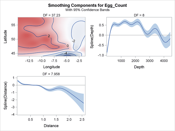
The smoothing component panel in Output 42.3.4 contains a contour for the spatial effect by Longitude and Latitude and two fitted univariate splines for Depth and Latitude, all demonstrating significantly nonlinear structures.
Output 42.3.4: Smoothing Components Panel
Overdispersion sometimes occurs for count data. One way to measure whether the data are overdispersed is to determine whether
Pearson’s chi-square divided by the error degrees of freedom is much larger than 1. You can compute that statistic by taking
the sum of squares of the Pearson residuals in the MackerelOut1 data set and then dividing that sum by the error degrees of freedom that is reported in Output 42.3.2. The computed value is approximately 8, which is much larger than 1, indicating the existence of overdispersion in this data
set.
There are many ways to solve the overdispersion problem. One approach is to fit a negative binomial distribution in which the variance of the mean contains a dispersion parameter. The following statements use PROC GAMPL to fit the nonparametric negative binomial regression model:
proc gampl data=Mackerel plots seed=2345;
   model Egg_Count = spline(Longitude Latitude/maxdf=40)
                     spline(Depth) spline(Distance)
                      / offset=Log_Net_Area dist=negbin;
   output out=MackerelOut2 pred=Pred2 pearson=Pea2;
run;
Output 42.3.5 displays the summary statistics from the negative binomial model. The model’s effective degrees of freedom is less than that of the Poisson model, even though the dispersion parameter costs one extra degree of freedom to fit. The values of the information criteria are also much less, indicating a better fit.
Output 42.3.5: Fit Statistics
| Mackerel Egg Density Study |
| Fit Statistics | |
|---|---|
| Penalized Log Likelihood | -1559.27838 |
| Roughness Penalty | 17.31664 |
| Effective Degrees of Freedom | 43.04281 |
| Effective Degrees of Freedom for Error | 586.85164 |
| AIC (smaller is better) | 3187.32573 |
| AICC (smaller is better) | 3193.75239 |
| BIC (smaller is better) | 3378.95442 |
| UBRE (smaller is better) | 0.55834 |
The “Tests for Smoothing Components” table in Output 42.3.6 shows that all spline terms are significant.
Output 42.3.6: Tests for Smoothing Components
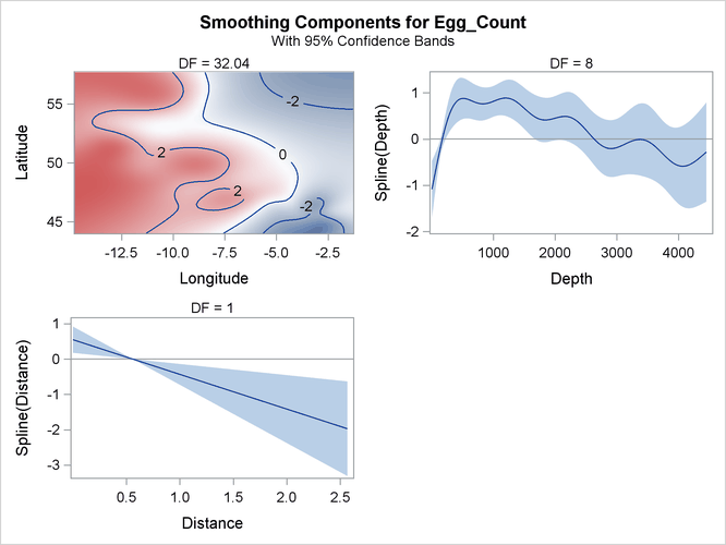
The smoothing component panel in Output 42.3.7 contains a fitted surface and curves for the three spline terms. Compared to the Poisson model, the fitted surface and curves are smoother. It is possible that the nonlinear dependency structure becomes smoother after its partial variations are accounted for by the dispersion parameter.
Output 42.3.7: Smoothing Components Panel
Pearson’s chi-square divided by the error degrees of freedom for the negative binomial model is approximately 1.5, which is close to 1. This suggests that the negative binomial model explains the overdispersion in the data.
The following DATA step and statements visualize the contours of mackerel egg density for both Poisson and negative binomial models:
data SurfaceFit;
   set Mackerel(keep=Longitude Latitude Net_Area Egg_Count);
   set MackerelOut1(keep=Pred1);
   set MackerelOut2(keep=Pred2);
   Pred1 = Pred1 / Net_Area;
   Pred2 = Pred2 / Net_Area;
run;
%let eopt = location=outside valign=top textattrs=graphlabeltext;
proc template;
   define statgraph surfaces;
      begingraph / designheight=360px;
         layout lattice / columns=2;
            layout overlay / &off0;
               entry "Poisson Model" / &eopt;
               contourplotparm z=Pred1 y=Latitude x=Longitude /
                               gridded=FALSE;
            endlayout;
            layout overlay / &off0;
               entry "Negative Binomial Model" / &eopt;
               contourplotparm z=Pred2 y=Latitude x=Longitude /
                               gridded=FALSE;
            endlayout;
         endlayout;
      endgraph;
   end;
run;

proc sgrender data=SurfaceFit template=surfaces;
run;
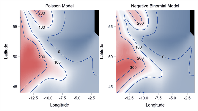
Output 42.3.8 displays two fitted surfaces from the Poisson model and the negative binomial model, respectively.
Output 42.3.8: Fitted Surfaces from Poisson Model and Negative Binomial Model