The TPSPLINE Procedure

Example 92.4 Large Data Set Application
This example illustrates how you can use the D= option to decrease the computation time needed by the TPSPLINE procedure. Although the D= option can be helpful in decreasing computation time for large data sets, it might produce unexpected results when used with small data sets.
The following statements generate the data set large:
data large;
   do x=-5 to 5 by 0.02;
      y=5*sin(3*x)+1*rannor(57391);
      output;
   end;
run;
The data set large contains 501 observations with one independent variable x and one dependent variable y. The following statements invoke PROC TPSPLINE to produce a thin-plate smoothing spline estimate and the associated  confidence interval. The output statistics are saved in the data set fit1.
proc tpspline data=large;
   model y  =(x) /lognlambda=(-5 to -1 by 0.2) alpha=0.01;
   output out=fit1 pred lclm uclm;
run;
The results from this MODEL statement are displayed in Output 92.4.1.
| Raw Data |
| Summary of Input Data Set | |
|---|---|
| Number of Non-Missing Observations | 501 |
| Number of Missing Observations | 0 |
| Unique Smoothing Design Points | 501 |
| Summary of Final Model | |
|---|---|
| Number of Regression Variables | 0 |
| Number of Smoothing Variables | 1 |
| Order of Derivative in the Penalty | 2 |
| Dimension of Polynomial Space | 2 |
| GCV Function | ||
|---|---|---|
| log10(n*Lambda) | GCV | |
| -5.000000 | 1.258653 | |
| -4.800000 | 1.228743 | |
| -4.600000 | 1.205835 | |
| -4.400000 | 1.188371 | |
| -4.200000 | 1.174644 | |
| -4.000000 | 1.163102 | |
| -3.800000 | 1.152627 | |
| -3.600000 | 1.142590 | |
| -3.400000 | 1.132700 | |
| -3.200000 | 1.122789 | |
| -3.000000 | 1.112755 | |
| -2.800000 | 1.102642 | |
| -2.600000 | 1.092769 | |
| -2.400000 | 1.083779 | |
| -2.200000 | 1.076636 | |
| -2.000000 | 1.072763 | * |
| -1.800000 | 1.074636 | |
| -1.600000 | 1.087152 | |
| -1.400000 | 1.120339 | |
| -1.200000 | 1.194023 | |
| -1.000000 | 1.344213 | |
| Summary Statistics of Final Estimation | |
|---|---|
| log10(n*Lambda) | -1.9483 |
| Smoothing Penalty | 9953.7066 |
| Residual SS | 475.0984 |
| Tr(I-A) | 471.0861 |
| Model DF | 29.9139 |
| Standard Deviation | 1.0042 |
| GCV | 1.0726 |
The following statements specify an identical model, but with the additional specification of the D= option. The estimates are obtained by treating nearby points as replicates.
proc tpspline data=large;
   model y  =(x) /lognlambda=(-5 to -1 by 0.2) d=0.05 alpha=0.01;
   output out=fit2 pred lclm uclm;
run;
The output is displayed in Output 92.4.2.
| Raw Data |
| Summary of Input Data Set | |
|---|---|
| Number of Non-Missing Observations | 501 |
| Number of Missing Observations | 0 |
| Unique Smoothing Design Points | 251 |
| Summary of Final Model | |
|---|---|
| Number of Regression Variables | 0 |
| Number of Smoothing Variables | 1 |
| Order of Derivative in the Penalty | 2 |
| Dimension of Polynomial Space | 2 |
| GCV Function | ||
|---|---|---|
| log10(n*Lambda) | GCV | |
| -5.000000 | 1.306536 | |
| -4.800000 | 1.261692 | |
| -4.600000 | 1.226881 | |
| -4.400000 | 1.200060 | |
| -4.200000 | 1.179284 | |
| -4.000000 | 1.162776 | |
| -3.800000 | 1.149072 | |
| -3.600000 | 1.137120 | |
| -3.400000 | 1.126220 | |
| -3.200000 | 1.115884 | |
| -3.000000 | 1.105766 | |
| -2.800000 | 1.095730 | |
| -2.600000 | 1.085972 | |
| -2.400000 | 1.077066 | |
| -2.200000 | 1.069954 | |
| -2.000000 | 1.066076 | * |
| -1.800000 | 1.067929 | |
| -1.600000 | 1.080419 | |
| -1.400000 | 1.113564 | |
| -1.200000 | 1.187172 | |
| -1.000000 | 1.337252 | |
| Summary Statistics of Final Estimation | |
|---|---|
| log10(n*Lambda) | -1.9477 |
| Smoothing Penalty | 9943.5618 |
| Residual SS | 472.1424 |
| Tr(I-A) | 471.0901 |
| Model DF | 29.9099 |
| Standard Deviation | 1.0011 |
| GCV | 1.0659 |
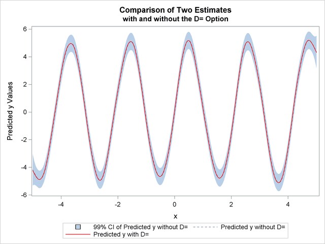
The difference between the two estimates is minimal. However, the CPU time for the second MODEL statement is only about  of the CPU time used in the first model fit.
The following statements produce a plot for comparison of the two estimates:
data fit2;
   set fit2;
   P1_y     = P_y;
   LCLM1_y  = LCLM_y;
   UCLM1_y  = UCLM_y;
   drop P_y LCLM_y UCLM_y;

proc sort data=fit1;
   by x y;
proc sort data=fit2;
   by x y;

data comp;
   merge fit1 fit2;
      by x y;
   label p1_y   ="Yhat1" p_y="Yhat0"
         lclm_y ="Lower CL"
         uclm_y ="Upper CL";

ods graphics on;
proc sgplot data=comp;
   title "Comparison of Two Estimates";
   title2 "with and without the D= Option";

   yaxis label="Predicted y Values";
   xaxis label="x";

   band x=x lower=lclm_y upper=uclm_y /name="range"
                      legendlabel="99% CI of Predicted y without D=";
   series x=x y=P_y/ name="P_y" legendlabel="Predicted y without D="
                      lineattrs=graphfit(thickness=1px pattern=shortdash);
   series x=x y=P1_y/ name="P1_y" legendlabel="Predicted y with D="
                      lineattrs=graphfit(thickness=1px color=red);
   discretelegend "range" "P_y" "P1_y";
run;
ods graphics off;
The estimates from fit1 and fit2 are displayed in Output 92.4.3 with the confidence interval from the fit1 output data set.