The TPSPLINE Procedure

Example 92.3 Multiple Minima of the GCV Function

The data in this example represent the deposition of sulfate (SO) at sites in the contiguous states of the United States in 1990. Each observation records the latitude and longitude of the site in addition to the SO deposition at the site measured in grams per square meter ().

You can use PROC TPSPLINE to fit a surface that reflects the general trend and that reveals underlying features of the data, which are shown in the following DATA step:

data so4;
input latitude longitude so4 @@;
datalines;
32.45833  87.24222 1.403 34.28778  85.96889 2.103
33.07139 109.86472 0.299 36.07167 112.15500 0.304
31.95056 112.80000 0.263 33.60500  92.09722 1.950

   ... more lines ...   

43.87333 104.19222 0.306 44.91722 110.42028 0.210
45.07611  72.67556 2.646
;

data pred;
   do latitude = 25 to 47 by 1;
      do longitude = 68 to 124 by 1;
         output;
      end;
   end;
run;

The preceding statements create the SAS data set so4 and the data set pred in order to make predictions on a regular grid. The following statements fit a surface for SO deposition. The ODS OUTPUT statement creates a data set called GCV to contain the GCV values for in the range from to .

ods graphics on;
proc tpspline data=so4 plots(only)=criterion;
   model so4 = (latitude longitude) /lognlambda=(-6 to 1 by 0.1);
   score data=pred out=prediction1;
run;

Partial output from these statements is displayed in Output 92.3.1 and Output 92.3.2.

Output 92.3.1 Partial Output from PROC TPSPLINE for Data Set SO

Raw Data

The TPSPLINE Procedure

Dependent Variable: so4

Summary of Input Data Set
Number of Non-Missing Observations	179
Number of Missing Observations	0
Unique Smoothing Design Points	179

Summary of Final Model
Number of Regression Variables	0
Number of Smoothing Variables	2
Order of Derivative in the Penalty	2
Dimension of Polynomial Space	3

Output 92.3.2 Partial Output from PROC TPSPLINE for Data Set SO

Summary Statistics of Final Estimation
log10(n*Lambda)	0.2770
Smoothing Penalty	2.4588
Residual SS	12.4450
Tr(I-A)	140.2750
Model DF	38.7250
Standard Deviation	0.2979
GCV	0.1132

Output 92.3.3 GCV Function of SO Data Set

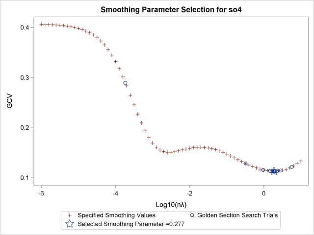
The GCV function has two minima. PROC TPSPLINE locates the global minimum at . The plot also displays a local minimum located around . The TPSPLINE procedure might not always find the global minimum, although it did in this case. If there is a predetermined search range based on prior knowledge, you can use the RANGE= option to narrow the search range in order to find a desired smoothing value. For example, if you believe a better smoothing parameter should be within the range, you can obtain the model with 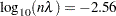with the following statements.

proc tpspline data=so4;
   model so4 = (latitude longitude) / range=(-4,-2);
   score data=pred out=prediction2;
run;

Output 92.3.4 displays the output from PROC TPSPLINE with a specified search range from the smoothing parameter.

Output 92.3.4 Output from PROC TPSPLINE for Data Set SO with

Raw Data

The TPSPLINE Procedure

Dependent Variable: so4

Summary of Input Data Set
Number of Non-Missing Observations	179
Number of Missing Observations	0
Unique Smoothing Design Points	179

Summary of Final Model
Number of Regression Variables	0
Number of Smoothing Variables	2
Order of Derivative in the Penalty	2
Dimension of Polynomial Space	3

Summary Statistics of Final Estimation
log10(n*Lambda)	-2.5600
Smoothing Penalty	177.2160
Residual SS	0.0438
Tr(I-A)	7.2083
Model DF	171.7917
Standard Deviation	0.0779
GCV	0.1508

The smoothing penalty in Output 92.3.4 is much larger than that displayed in Output 92.3.2. The estimate in Output 92.3.2 uses a large value; therefore, the surface is smoother than the estimate by using (Output 92.3.4).

The estimate based on has a larger value of degrees of freedom, and it has a much smaller standard deviation.

However, a smaller standard deviation in nonparametric regression does not necessarily mean that the estimate is good: a small value always produces an estimate closer to the data and, therefore, a smaller standard deviation.

When ODS Graphics is enabled, you can compare the two fits by supplying and to the LOGNLAMBDA= option:

proc tpspline data=so4;
   model so4 = (latitude longitude) / lognlambda=(0.277 -2.56);
run;

Output 92.3.5 shows the contour surfaces of two models with the two minima. The fit that corresponds to the global minimum shows a smoother fit that captures the general structure in the data set. The fit at the local minimum is a rougher fit that captures local details. The response values are also displayed as circles with the same color gradient by the default GRADIENT contour-option. The contrast between the predicted and observed SO deposition is greater for the smoother fit than for the other one, which means the smoother fit has larger absolute residual values.

Output 92.3.5 Panel of Contour Fit Plots by and

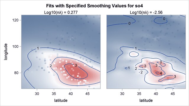
The residuals for the two fits can be visualized in RESIDUALBYSMOOTH panels. Output 92.3.6 is a panel of plots of residuals against smoothing variable Latitude. Output 92.3.7 is a panel of plots of residuals against smoothing variable Longitude. Both panels show that the residuals from the model with the global minimum are larger in absolute values than the ones from the local minimum. This is expected, since the optimal model achieves the smallest GCV value by significantly increasing the smoothness of fit and sacrificing a little in the goodness of fit.

Output 92.3.6 Panel of Residuals by Latitude Plots

Output 92.3.7 Panel of Residuals by Longitude Plots

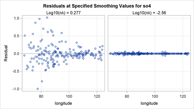
In summary, the fit with represents the underlying surface, while the fit with the overfits the data and captures the additional noise component.