The TPSPLINE Procedure

| Computational Formulas |
The theoretical foundations for the thin-plate smoothing spline are described in Duchon (1976, 1977) and Meinguet (1979). Further results and applications are given in Wahba and Wendelberger (1980), Hutchinson and Bischof (1983), and Seaman and Hutchinson (1985).
Suppose that  is a space of functions whose partial derivatives of total order
  are in
  , where
  is the domain of
  .
.
Now, consider the data model
 |
where  .
.
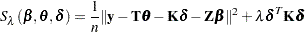
Using the notation from the section Penalized Least Squares Estimation, for a fixed  , estimate
  by minimizing the penalized least squares function
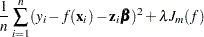 |
 is the penalty term to enforce smoothness on . There are several ways to define
  . For the thin-plate smoothing spline, with
  of dimension
  , define as
 |
where  . Under this definition, gives zero penalty to some functions. The space that is spanned by the set of polynomials that contribute zero penalty is called the polynomial space. The dimension of the polynomial space
  is a function of dimension and order of the smoothing penalty,
  .
.
Given the condition that  , the function that minimizes the penalized least squares criterion has the form
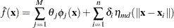 |
where  and
and  are vectors of coefficients to be estimated. The functions
  are linearly independent polynomials that span the space of functions for which is zero. The basis functions
  are defined as
 |
When  and
and  , then
  ,
,  ,
,  , and
, and  . is as follows:
 |
For the sake of simplicity, the formulas and equations that follow assume . See Wahba (1990) and Bates et al. (1987) for more details.
Duchon (1976) showed that  can be represented as
 |
where 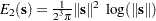 for . For derivations of
  for other values of , see Villalobos and Wahba (1987).
If you define  with elements
 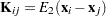 and
and  with elements
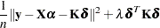
  , the goal is to find vectors of coefficients
  and that minimize
 |
A unique solution is guaranteed if the matrix  is of full rank and
  .
.
If  and
and  , the expression for
  becomes
 |
The coefficients  and
and  can be obtained by solving
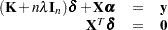 |
To compute  and , let the QR decomposition of
  be
be
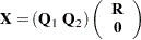 |
where  is an orthogonal matrix and
  is an upper triangular, with
  (Dongarra et al. 1979).
Since  , must be in the column space of
  . Therefore, can be expressed as
  for a vector
  . Substituting
  into the preceding equation and multiplying through by
  gives
gives
 |
or
 |
The coefficient can be obtained by solving
 |
The influence matrix  is defined as
 |
and has the form
 |
Similar to the regression case, if you consider the trace of  as the degrees of freedom for the model and the trace of
  as the degrees of freedom for the error, the estimate
  can be represented as
 |
where  is the residual sum of squares. Theoretical properties of these estimates have not yet been published. However, good numerical results in simulation studies have been described by several authors. For more information, see O’Sullivan and Wong (1987), Nychka (1986a, 1986b, 1988), and Hall and Titterington (1987).
Confidence Intervals
Viewing the spline model as a Bayesian model, Wahba (1983) proposed Bayesian confidence intervals for smoothing spline estimates as
 |
where  is the
  th diagonal element of the matrix and
  is the
  quantile of the standard normal distribution. The confidence intervals are interpreted as intervals "across the function" as opposed to pointwise intervals.
For SCORE data sets, the hat matrix is not available. To compute the Bayesian confidence interval for a new point  , let
, let
 |
and let  be an
be an  vector with th entry
 |
When and ,  is computed with
 |
 is a vector of evaluations of by the polynomials that span the functional space where is zero. The details for ,
  , and
, and  are discussed in the previous section. Wahba (1983) showed that the Bayesian posterior variance of satisfies
 |
where
 |
 |
 |
|||
 |
|
 |
Suppose that you fit a spline estimate that consists of a true function and a random error term  to experimental data. In repeated experiments, it is likely that about
  of the confidence intervals cover the corresponding true values, although some values are covered every time and other values are not covered by the confidence intervals most of the time. This effect is more pronounced when the true surface or surface has small regions of particularly rapid change.
Smoothing Parameter
The quantity is called the smoothing parameter, which controls the balance between the goodness of fit and the smoothness of the final estimate.
A large heavily penalizes the th derivative of the function, thus forcing  close to 0. A small places less of a penalty on rapid change in
  , resulting in an estimate that tends to interpolate the data points.
The smoothing parameter greatly affects the analysis, and it should be selected with care. One method is to perform several analyses with different values for and compare the resulting final estimates.
A more objective way to select the smoothing parameter is to use the "leave-out-one" cross validation function, which is an approximation of the predicted mean squares error. A generalized version of the leave-out-one cross validation function is proposed by Wahba (1990) and is easy to calculate. This generalized cross validation (GCV) function is defined as
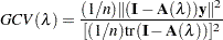 |
The justification for using the GCV function to select relies on asymptotic theory. Thus, you cannot expect good results for very small sample sizes or when there is not enough information in the data to separate the model from the error component. Simulation studies suggest that for independent and identically distributed Gaussian noise, you can obtain reliable estimates of for  greater than
  or
or  . Note that, even for large values of (say,
  ), in extreme Monte Carlo simulations there might be a small percentage of unwarranted extreme estimates in which
  or
or  (Wahba 1983). Generally, if is known to within an order of magnitude, the occasional extreme case can be readily identified. As gets larger, the effect becomes weaker.
The GCV function is fairly robust against nonhomogeneity of variances and non-Gaussian errors (Villalobos and Wahba 1987). Andrews (1988) has provided favorable theoretical results when variances are unequal. However, this selection method is likely to give unsatisfactory results when the errors are highly correlated.
The GCV value might be suspect when is extremely small because computed values might become indistinguishable from zero. In practice, calculations with  or near 0 can cause numerical instabilities that result in an unsatisfactory solution. Simulation studies have shown that a with
  is small enough that the final estimate based on this almost interpolates the data points. A GCV value based on a
  might not be accurate.