The TPSPLINE Procedure

Getting Started: TPSPLINE Procedure
The following example demonstrates how you can use the TPSPLINE procedure to fit a semiparametric model.
Suppose that y is a continuous variable and x1 and x2 are two explanatory variables of interest. To fit a bivariate thin-plate spline model, you can use a MODEL statement similar to that used in many regression procedures in the SAS System:
proc tpspline;
    model y = (x1 x2);
run;
The TPSPLINE procedure can fit semiparametric models; the parentheses in the preceding MODEL statement separate the smoothing variables from the regression variables. The following statements illustrate this syntax:
proc tpspline;
    model y = z1 (x1 x2);
run;
This model assumes a linear relation with z1 and an unknown functional relation with x1 and x2.
If you want to fit several responses by using the same explanatory variables, you can save computation time by using the multiple responses feature in the MODEL statement. For example, if y1 and y2 are two response variables, the following MODEL statement can be used to fit two models. Separate analyses are then performed for each response variable.
proc tpspline;
    model y1 y2 = (x1 x2);
run;
The following example illustrates the use of PROC TPSPLINE. The data are from Bates et al. (1987).
data Measure;
    input x1 x2 y @@;
datalines;
-1.0 -1.0   15.54483570   -1.0 -1.0    15.76312613
 -.5 -1.0   18.67397826    -.5 -1.0    18.49722167
  .0 -1.0   19.66086310     .0 -1.0    19.80231311
  .5 -1.0   18.59838649     .5 -1.0    18.51904737
 1.0 -1.0   15.86842815    1.0 -1.0    16.03913832
-1.0  -.5   10.92383867   -1.0  -.5    11.14066546
 -.5  -.5   14.81392847    -.5  -.5    14.82830425
  .0  -.5   16.56449698     .0  -.5    16.44307297
  .5  -.5   14.90792284     .5  -.5    15.05653924
 1.0  -.5   10.91956264    1.0  -.5    10.94227538
-1.0   .0    9.61492010   -1.0   .0     9.64648093
 -.5   .0   14.03133439    -.5   .0    14.03122345
  .0   .0   15.77400253     .0   .0    16.00412514
  .5   .0   13.99627680     .5   .0    14.02826553
 1.0   .0    9.55700164    1.0   .0     9.58467047
-1.0   .5   11.20625177   -1.0   .5    11.08651907
 -.5   .5   14.83723493    -.5   .5    14.99369172
  .0   .5   16.55494349     .0   .5    16.51294369
  .5   .5   14.98448603     .5   .5    14.71816070
 1.0   .5   11.14575565    1.0   .5    11.17168689
-1.0  1.0   15.82595514   -1.0  1.0    15.96022497
 -.5  1.0   18.64014953    -.5  1.0    18.56095997
  .0  1.0   19.54375504     .0  1.0    19.80902641
  .5  1.0   18.56884576     .5  1.0    18.61010439
 1.0  1.0   15.86586951    1.0  1.0    15.90136745
;
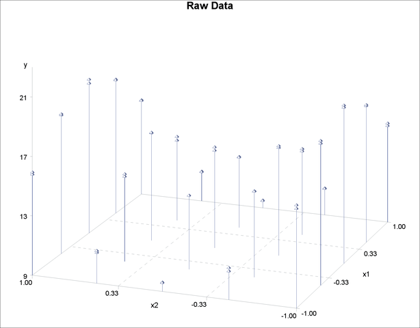
The data set Measure contains three variables x1, x2, and y. Suppose that you want to fit a surface by using the variables x1 and x2 to model the response y. The variables x1 and x2 are spaced evenly on a  square, and the response y is generated by adding a random error to a function
  . The raw data are plotted in three-dimensional scatter plot by using the G3D procedure. In order to visualize those replicates, half of the data are shifted a little bit by adding a small value (
 ) to x1 values, as in the following statements:
data Measure1;
   set Measure;
run;

proc sort data=Measure1;
   by x2 x1;
run;

data Measure1;
   set Measure1;
   if mod(_N_, 2) = 0 then x1=x1+0.001;
run;
proc g3d data=Measure1;
   scatter x2*x1=y /size=.5
                    zmin=9 zmax=21
                    zticknum=4;
   title "Raw Data";
run;
Figure 92.1 displays the raw data.
The following statements invoke the TPSPLINE procedure, by using the Measure data set as input. In the MODEL statement, the x1 and x2 variables are listed as smoothing variables. The LOGNLAMBDA= option specifies that PROC TPSPLINE examine a list of models with  ranging from
  to
to  . The OUTPUT statement creates the data set estimate to contain the predicted values and the
  upper and lower confidence limits from the best model selected by the GCV criterion.
ods graphics on;
proc tpspline data=Measure;
   model y=(x1 x2) /lognlambda=(-4 to -2.5 by 0.1);
   output out=estimate pred uclm lclm;
run;

proc print data=estimate;
run;
When ODS Graphics is enabled, PROC TPSPLINE produces several default plots. One of the default plots is the contour plot of the fitted surface, shown in Figure 92.2. The surface exhibits nonlinear patterns along the directions of both predictors.
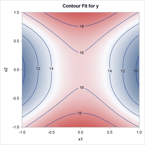
Figure 92.3 shows the “Criterion Plot” that provides a graphical display of the GCV selection process. Three sets of values are shown in the plot: the specified smoothing values and their GCV values, the examined smoothing values and their GCV values during the optimization process, and the best smoothing parameter and its GCV value. The final thin-plate smoothing spline estimate is based on 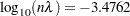 , which minimizes the GCV.
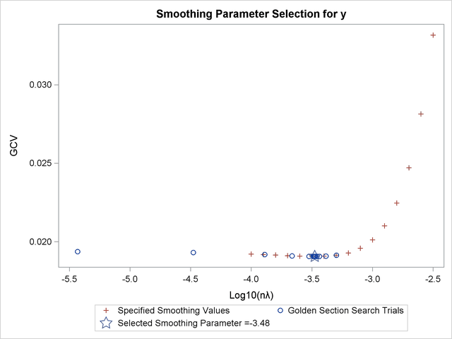
Figure 92.4 shows that the data set Measure contains  observations with
  unique design points. The final model contains no parametric regression terms and two smoothing variables. The order derivative in the penalty is
  by default, and the dimension of polynomial space is
  . See the section Computational Formulas for definitions.
Figure 92.4 also lists the GCV values along with the supplied values of . The value that minimizes the GCV function is  among the given list of .
The residual sum of squares from the fitted model is  , and the model degrees of freedom are
  . The standard deviation, defined as
  , is
, is  . The predictions and confidence limits are displayed in Figure 92.5.
| Raw Data |
| Summary of Input Data Set | |
|---|---|
| Number of Non-Missing Observations | 50 |
| Number of Missing Observations | 0 |
| Unique Smoothing Design Points | 25 |
| Summary of Final Model | |
|---|---|
| Number of Regression Variables | 0 |
| Number of Smoothing Variables | 2 |
| Order of Derivative in the Penalty | 2 |
| Dimension of Polynomial Space | 3 |
| GCV Function | ||
|---|---|---|
| log10(n*Lambda) | GCV | |
| -4.000000 | 0.019215 | |
| -3.900000 | 0.019183 | |
| -3.800000 | 0.019148 | |
| -3.700000 | 0.019113 | |
| -3.600000 | 0.019082 | |
| -3.500000 | 0.019064 | * |
| -3.400000 | 0.019074 | |
| -3.300000 | 0.019135 | |
| -3.200000 | 0.019286 | |
| -3.100000 | 0.019584 | |
| -3.000000 | 0.020117 | |
| -2.900000 | 0.021015 | |
| -2.800000 | 0.022462 | |
| -2.700000 | 0.024718 | |
| -2.600000 | 0.028132 | |
| -2.500000 | 0.033165 | |
| Summary Statistics of Final Estimation | |
|---|---|
| log10(n*Lambda) | -3.4762 |
| Smoothing Penalty | 2558.1432 |
| Residual SS | 0.2461 |
| Tr(I-A) | 25.4068 |
| Model DF | 24.5932 |
| Standard Deviation | 0.0984 |
| GCV | 0.0191 |
| Raw Data |
| Obs | x1 | x2 | y | P_y | LCLM_y | UCLM_y |
|---|---|---|---|---|---|---|
| 1 | -1.0 | -1.0 | 15.5448 | 15.6474 | 15.5115 | 15.7832 |
| 2 | -1.0 | -1.0 | 15.7631 | 15.6474 | 15.5115 | 15.7832 |
| 3 | -0.5 | -1.0 | 18.6740 | 18.5783 | 18.4430 | 18.7136 |
| 4 | -0.5 | -1.0 | 18.4972 | 18.5783 | 18.4430 | 18.7136 |
| 5 | 0.0 | -1.0 | 19.6609 | 19.7270 | 19.5917 | 19.8622 |
| 6 | 0.0 | -1.0 | 19.8023 | 19.7270 | 19.5917 | 19.8622 |
| 7 | 0.5 | -1.0 | 18.5984 | 18.5552 | 18.4199 | 18.6905 |
| 8 | 0.5 | -1.0 | 18.5190 | 18.5552 | 18.4199 | 18.6905 |
| 9 | 1.0 | -1.0 | 15.8684 | 15.9436 | 15.8077 | 16.0794 |
| 10 | 1.0 | -1.0 | 16.0391 | 15.9436 | 15.8077 | 16.0794 |
| 11 | -1.0 | -0.5 | 10.9238 | 11.0467 | 10.9114 | 11.1820 |
| 12 | -1.0 | -0.5 | 11.1407 | 11.0467 | 10.9114 | 11.1820 |
| 13 | -0.5 | -0.5 | 14.8139 | 14.8246 | 14.6896 | 14.9597 |
| 14 | -0.5 | -0.5 | 14.8283 | 14.8246 | 14.6896 | 14.9597 |
| 15 | 0.0 | -0.5 | 16.5645 | 16.5102 | 16.3752 | 16.6452 |
| 16 | 0.0 | -0.5 | 16.4431 | 16.5102 | 16.3752 | 16.6452 |
| 17 | 0.5 | -0.5 | 14.9079 | 14.9812 | 14.8461 | 15.1162 |
| 18 | 0.5 | -0.5 | 15.0565 | 14.9812 | 14.8461 | 15.1162 |
| 19 | 1.0 | -0.5 | 10.9196 | 10.9497 | 10.8144 | 11.0850 |
| 20 | 1.0 | -0.5 | 10.9423 | 10.9497 | 10.8144 | 11.0850 |
| 21 | -1.0 | 0.0 | 9.6149 | 9.6372 | 9.5019 | 9.7724 |
| 22 | -1.0 | 0.0 | 9.6465 | 9.6372 | 9.5019 | 9.7724 |
| 23 | -0.5 | 0.0 | 14.0313 | 14.0188 | 13.8838 | 14.1538 |
| 24 | -0.5 | 0.0 | 14.0312 | 14.0188 | 13.8838 | 14.1538 |
| 25 | 0.0 | 0.0 | 15.7740 | 15.8822 | 15.7472 | 16.0171 |
| 26 | 0.0 | 0.0 | 16.0041 | 15.8822 | 15.7472 | 16.0171 |
| 27 | 0.5 | 0.0 | 13.9963 | 14.0006 | 13.8656 | 14.1356 |
| 28 | 0.5 | 0.0 | 14.0283 | 14.0006 | 13.8656 | 14.1356 |
| 29 | 1.0 | 0.0 | 9.5570 | 9.5769 | 9.4417 | 9.7122 |
| 30 | 1.0 | 0.0 | 9.5847 | 9.5769 | 9.4417 | 9.7122 |
| 31 | -1.0 | 0.5 | 11.2063 | 11.1614 | 11.0261 | 11.2967 |
| 32 | -1.0 | 0.5 | 11.0865 | 11.1614 | 11.0261 | 11.2967 |
| 33 | -0.5 | 0.5 | 14.8372 | 14.9182 | 14.7831 | 15.0532 |
| 34 | -0.5 | 0.5 | 14.9937 | 14.9182 | 14.7831 | 15.0532 |
| 35 | 0.0 | 0.5 | 16.5549 | 16.5386 | 16.4036 | 16.6736 |
| 36 | 0.0 | 0.5 | 16.5129 | 16.5386 | 16.4036 | 16.6736 |
| 37 | 0.5 | 0.5 | 14.9845 | 14.8549 | 14.7199 | 14.9900 |
| 38 | 0.5 | 0.5 | 14.7182 | 14.8549 | 14.7199 | 14.9900 |
| 39 | 1.0 | 0.5 | 11.1458 | 11.1727 | 11.0374 | 11.3080 |
| 40 | 1.0 | 0.5 | 11.1717 | 11.1727 | 11.0374 | 11.3080 |
| 41 | -1.0 | 1.0 | 15.8260 | 15.8851 | 15.7493 | 16.0210 |
| 42 | -1.0 | 1.0 | 15.9602 | 15.8851 | 15.7493 | 16.0210 |
| 43 | -0.5 | 1.0 | 18.6401 | 18.5946 | 18.4593 | 18.7299 |
| 44 | -0.5 | 1.0 | 18.5610 | 18.5946 | 18.4593 | 18.7299 |
| 45 | 0.0 | 1.0 | 19.5438 | 19.6729 | 19.5376 | 19.8081 |
| 46 | 0.0 | 1.0 | 19.8090 | 19.6729 | 19.5376 | 19.8081 |
| 47 | 0.5 | 1.0 | 18.5688 | 18.5832 | 18.4478 | 18.7185 |
| 48 | 0.5 | 1.0 | 18.6101 | 18.5832 | 18.4478 | 18.7185 |
| 49 | 1.0 | 1.0 | 15.8659 | 15.8761 | 15.7402 | 16.0120 |
| 50 | 1.0 | 1.0 | 15.9014 | 15.8761 | 15.7402 | 16.0120 |
You can also use the TEMPLATE and SGRENDER procedures to create a perspective plot for visualizing the fitted surface. Because the data in the data set Measure are very sparse, the fitted surface is not smooth. To produce a smoother surface, the following statements generate the data set pred in order to obtain a finer grid. The LOGNLAMBDA0= option requests that PROC TPSPLINE fit a model with a fixed value of  . The SCORE statement evaluates the fitted surface at those new design points.
data pred;
   do x1=-1 to 1 by 0.1;
      do x2=-1 to 1 by 0.1;
         output;
      end;
   end;
run;

proc tpspline data=measure;
   model y=(x1 x2)/lognlambda0=-3.4762;
   score data=pred out=predy;
run;

proc template;
    define statgraph surface;
    dynamic _X _Y _Z _T;
    begingraph /designheight=360;
        entrytitle _T;
        layout overlay3d/rotate=120 cube=false  xaxisopts=(label="x1")
                         yaxisopts=(label="x2") zaxisopts=(label="P_y");
                         surfaceplotparm x=_X y=_Y z=_Z;
        endlayout;
    endgraph;
    end;
run;

proc sgrender data=predy template=surface;
    dynamic _X='x1' _Y='x2' _Z='P_y'
            _T='Plot of Fitted Surface on a Fine Grid';
run;
The surface plot based on the finer grid is displayed in Figure 92.6. The plot indicates that a parametric model with quadratic terms of x1 and x2 provides a reasonable fit to the data.
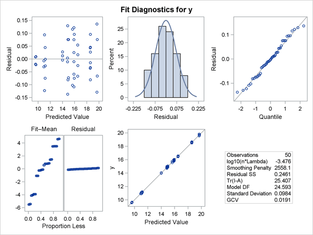
Figure 92.7 shows a panel of fit diagnostics for the selected model that indicate a reasonable fit:
The predicted values closely approximate the observed values.
The residuals are approximately normally distributed and do not show obvious systematic patterns.
The RFPLOT shows that much variation in the response variable is addressed by the fit and only a little remains in the residuals.