The TPSPLINE Procedure

| Penalized Least Squares Estimation |
Penalized least squares estimation provides a way to balance fitting the data closely and avoiding excessive roughness or rapid variation. A penalized least squares estimate is a surface that minimizes the penalized least squares over the class of all surfaces that satisfy sufficient regularity conditions.
Define  as a
as a  -dimensional covariate vector from an
  matrix
  ,
,  as a
as a  -dimensional covariate vector, and
  as the observation associated with
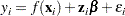
  . Assuming that the relation between and is linear but the relation between and is unknown, you can fit the data by using a semiparametric model as follows:
 |
where  is an unknown function that is assumed to be reasonably smooth,
  , are independent, zero-mean random errors, and
  is a -dimensional unknown parametric vector.
This model consists of two parts. The  is the parametric part of the model, and the are the regression variables. The
  is the nonparametric part of the model, and the are the smoothing variables. The ordinary least squares method estimates
  and by minimizing the quantity:
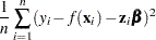 |
However, the functional space of  is so large that you can always find a function that interpolates the data points. In order to obtain an estimate that fits the data well and has some degree of smoothness, you can use the penalized least squares method.
The penalized least squares function is defined as
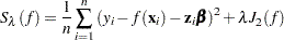 |
where  is the penalty on the roughness of and is defined, in most cases, as the integral of the square of the second derivative of .
The first term measures the goodness of fit and the second term measures the smoothness associated with . The  term is the smoothing parameter, which governs the tradeoff between smoothness and goodness of fit. When is large, it more heavily penalizes rougher fits. Conversely, a small value of puts more emphasis on the goodness of fit.
The estimate  is selected from a reproducing kernel Hilbert space, and it can be represented as a linear combination of a sequence of basis functions. Hence, the final estimates of can be written as
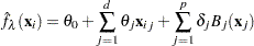 |
where  is the basis function, which depends on where the data
  are located, and
  and
and  are the coefficients that need to be estimated.
For a fixed , the coefficients  can be estimated by solving an
  system.
The smoothing parameter can be chosen by minimizing the generalized cross validation (GCV) function.
If you write
 |
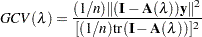
then  is referred to as the hat or smoothing matrix, and the GCV function
  is defined as
 |