The TPSPLINE Procedure

Example 92.1 Partial Spline Model Fit
This example analyzes the data set Measure that was introduced in the section Getting Started: TPSPLINE Procedure. That analysis determined that the final estimated surface can be represented by a quadratic function for one or both of the independent variables. This example illustrates how you can use PROC TPSPLINE to fit a partial spline model. The data set Measure is fit by using the following model:
 |
The model has a parametric component (associated with the  variable) and a nonparametric component (associated with the
  variable). The following statements fit a partial spline model:
data Measure;
   set Measure;
   x1sq = x1*x1;
run;

data pred;
   do x1=-1 to 1 by 0.1;
      do x2=-1 to 1 by 0.1;
         x1sq = x1*x1;
         output;
      end;
   end;
run;

proc tpspline data= measure;
   model y = x1 x1sq (x2);
   score data = pred out  = predy;
run;
Output 92.1.1 displays the results from these statements.
| Raw Data |
| Summary of Input Data Set | |
|---|---|
| Number of Non-Missing Observations | 50 |
| Number of Missing Observations | 0 |
| Unique Smoothing Design Points | 5 |
| Summary of Final Model | |
|---|---|
| Number of Regression Variables | 2 |
| Number of Smoothing Variables | 1 |
| Order of Derivative in the Penalty | 2 |
| Dimension of Polynomial Space | 4 |
| Summary Statistics of Final Estimation | |
|---|---|
| log10(n*Lambda) | -2.2374 |
| Smoothing Penalty | 205.3461 |
| Residual SS | 8.5821 |
| Tr(I-A) | 43.1534 |
| Model DF | 6.8466 |
| Standard Deviation | 0.4460 |
| GCV | 0.2304 |
As displayed in Output 92.1.1, there are five unique design points for the smoothing variable and two regression variables in the model  . The dimension of the polynomial space is
  . The standard deviation of the estimate is much larger than the one based on the model with both and as smoothing variables (
 compared to
  ). One of the many possible explanations might be that the number of unique design points of the smoothing variable is too small to warrant an accurate estimate for
  .
.
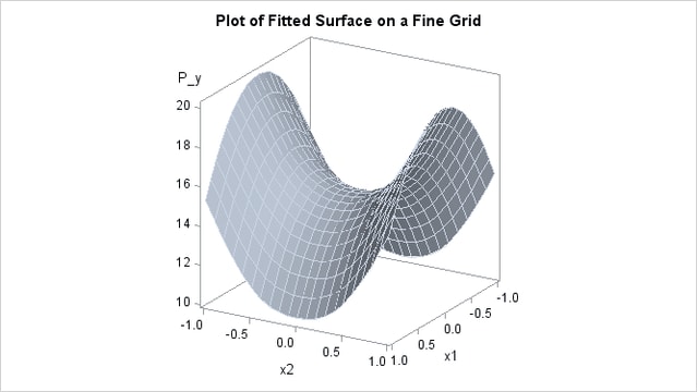
The following statements produce a surface plot for the partial spline model by using the surface template that is defined in the section Getting Started: TPSPLINE Procedure.
ods graphics on;

proc sgrender data=predy template=surface;
    dynamic _X='x1' _Y='x2' _Z='P_y' _T='Plot of Fitted Surface on a Fine Grid';
run;

ods graphics off;
The surface displayed in Output 92.1.2 is similar to the one estimated by using the full nonparametric model (displayed in Output 92.2 and Output 92.6).