The HPQLIM Procedure

Heteroscedasticity
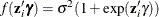
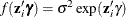
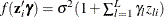
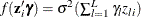
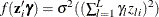
If the variance of regression disturbance, ( ), is heteroscedastic, the variance can be specified as a function of variables
![\[ E(\epsilon _{i}^{2}) = \sigma _{i}^{2} = f(\mb{z}_{i}’\bgamma ) \]](images/etsug_hpqlim0103.png)
Table 22.2 shows various functional forms of heteroscedasticity and the corresponding options to request each model.
Table 22.2: Specification Summary for Modeling Heteroscedasticity
|
Number |
Model |
Options |
|
|---|---|---|---|
|
1 |
|
LINK=EXP (default) |
|
|
2 |
|
LINK=EXP NOCONST |
|
|
3 |
|
LINK=LINEAR |
|
|
4 |
|
LINK=LINEAR SQUARE |
|
|
5 |
|
LINK=LINEAR NOCONST |
|
|
6 |
|
LINK=LINEAR SQUARE NOCONST |

In models 3 and 5, variances of some observations might be negative. Although the HPQLIM procedure assigns a large penalty to move the optimization away from such a region, the optimization might not be able to improve the objective function value and might become locked in the region. Signs of such an outcome include extremely small likelihood values or missing standard errors in the estimates. In models 2 and 6, variances are guaranteed to be greater than or equal to zero, but variances of some observations might be very close to 0. In these scenarios, standard errors might be missing. Models 1 and 4 do not have such problems. Variances in these models are always positive and never close to 0.
For more information, see the section Heteroscedasticity and Box-Cox Transformation.