The HPQLIM Procedure
Example 22.2 Bayesian High-Performance Model with Censoring
This example shows the use of the Bayesian analysis available in the HPQLIM procedure with an emphasis on processing a large data set and on the performance improvements that are achieved by executing in a high-performance distributed environment.
The model and the data set are the same as in Example 22.1, and the priors are set to the defaults.
The model is executed in the distributed computing environment with two threads and only one node. These settings are used to obtain a hypothetical environment that might resemble running the HPQLIM procedure on a desktop workstation with a dual-core CPU. To run the following statements successfully, you need to set the macro variables GRIDHOST and GRIDINSTALLLOC to resolve to appropriate values, or you can replace the references to the macro variables in the example with the appropriate values.
    option set=GRIDHOST="&GRIDHOST";
    option set=GRIDINSTALLLOC="&GRIDINSTALLLOC";
 proc hpqlim data=simulate ;
 bayes nbi=10000 nmc=30000;
    performance nthreads=2 nodes=1 details
                 host="&GRIDHOST" install="&GRIDINSTALLLOC";
    model y=x1-x7 /censored(lb=0 ub=400);
    %*;     ods output PerformanceInfo=perfInfo;
    %*;     ods output Timing=time;
run;
Output 22.2.1 shows a summary of the posterior distribution that is associated with the censored model when you use diffuse prior distributions.
Output 22.2.1: Posterior Summary for Bayesian Censored Model
| Estimating a Tobit model |
| Posterior Summaries | ||||||
|---|---|---|---|---|---|---|
| Parameter | N | Mean | Standard Deviation |
Percentiles | ||
| 25% | 50% | 75% | ||||
| Intercept | 30000 | 2.2168 | 0.2166 | 2.0682 | 2.2171 | 2.3674 |
| x1 | 30000 | 3.0656 | 0.1953 | 2.9356 | 3.0638 | 3.1974 |
| x2 | 30000 | 3.9936 | 0.2052 | 3.8572 | 3.9951 | 4.1308 |
| x3 | 30000 | 1.8496 | 0.2019 | 1.7201 | 1.8475 | 1.9813 |
| x4 | 30000 | 4.1637 | 0.1986 | 4.0295 | 4.1574 | 4.2996 |
| x5 | 30000 | -3.0226 | 0.1981 | -3.1603 | -3.0249 | -2.8848 |
| x6 | 30000 | -5.1776 | 0.1985 | -5.3099 | -5.1720 | -5.0456 |
| x7 | 30000 | -2.6889 | 0.1993 | -2.8235 | -2.6882 | -2.5523 |
| _Sigma | 30000 | 400.0 | 0.2623 | 399.8 | 400.0 | 400.2 |
Output 22.2.2 show a summary of the performance when you use a distributed computing environment with one node and two threads.
Output 22.2.2: Performance Analysis for Bayesian Censored Model on One Node with Two Threads
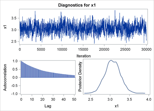
Finally, Output 22.2.3 shows the diagnostic and summary plots that are associated with X1.
Output 22.2.3: Bayesian Diagnostic and Summary Plots for x1

In the following statements, the PERFORMANCE statement is modified to use a grid with 10 nodes, where each node spawns eight threads:
    option set=GRIDHOST="&GRIDHOST";
    option set=GRIDINSTALLLOC="&GRIDINSTALLLOC";
 proc hpqlim data=simulate ;
 bayes nbi=10000 nmc=30000;
    performance nthreads=8 nodes=10 details
                 host="&GRIDHOST" install="&GRIDINSTALLLOC";
    model y=x1-x7 /censored(lb=0 ub=400);
    %*;     ods output PerformanceInfo=perfInfo;
    %*;     ods output Timing=time;
run;
The two models are identical, but the second implementation, which was run on a grid that used 10 nodes with eight threads each, took only 15.7 minutes instead of 12.8 hours to sample from the same posterior distribution.
Output 22.2.4: Performance Analysis for Bayesian Censored Model on Ten Nodes with Eight Threads Each
