The COUNTREG Procedure
- Overview
- Getting Started
-
Syntax
 Functional SummaryPROC COUNTREG StatementBAYES StatementBOUNDS StatementBY StatementCLASS StatementDISPMODEL StatementFREQ StatementINIT StatementMODEL StatementNLOPTIONS StatementOUTPUT StatementPERFORMANCE StatementPRIOR StatementRESTRICT StatementSCORE StatementSHOW StatementSPATIALDISPEFFECTS StatementSPATIALEFFECTS StatementSPATIALID StatementSPATIALZEROEFFECTS StatementSTORE StatementTEST StatementWEIGHT StatementZEROMODEL Statement
 -
DetailsSpecification of RegressorsMissing ValuesPoisson RegressionConway-Maxwell-Poisson RegressionNegative Binomial RegressionZero-Inflated Count Regression OverviewZero-Inflated Poisson RegressionZero-Inflated Conway-Maxwell-Poisson RegressionZero-Inflated Negative Binomial RegressionSpatial Lag of X ModelVariable SelectionPanel Data AnalysisBY Groups and Scoring with an Item StoreParameter Naming Conventions for the RESTRICT, TEST, BOUNDS, and INIT StatementsComputational ResourcesNonlinear Optimization OptionsCovariance Matrix TypesDisplayed OutputBayesian AnalysisPrior DistributionsAutomated MCMC AlgorithmMarginal LikelihoodOUTPUT OUT= Data SetOUTEST= Data SetODS Table NamesODS Graphics
-
Examples
- References
Marginal Likelihood
The Bayes theorem states that
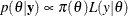
where  is a vector of parameters and
  is the product of the prior densities, which are specified in the PRIOR
statement. The term
is the product of the prior densities, which are specified in the PRIOR
statement. The term  is the likelihood associated with the MODEL
statement. The function
is the likelihood associated with the MODEL
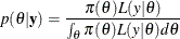
statement. The function  is the nonnormalized posterior distribution over the parameter vector . The normalized posterior distribution, or simply the posterior distribution, is
The denominator 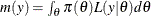 , also called the “marginal likelihood,” is a quantity of interest because it represents the probability of the data after
the effect of the parameter vector has been averaged out. Due to its interpretation, the marginal likelihood can be used in
various applications, including model averaging and variable or model selection.
, also called the “marginal likelihood,” is a quantity of interest because it represents the probability of the data after
the effect of the parameter vector has been averaged out. Due to its interpretation, the marginal likelihood can be used in
various applications, including model averaging and variable or model selection.
A natural estimate of the marginal likelihood is provided by the harmonic mean,
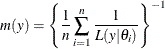
where  is a sample draw from the posterior distribution. This estimator has proven to be unstable in practical applications.
An alternative and more stable estimator can be obtained by using an importance sampling scheme. The auxiliary distribution for the importance sampler can be chosen through the cross-entropy theory (Chan and Eisenstat 2015). In particular, given a parametric family of distributions, the auxiliary density function is chosen to be the one closest, in terms of the Kullback-Leibler divergence, to the probability density that would give a zero variance estimate of the marginal likelihood. In practical terms, this is equivalent to the following algorithm:
-
Choose a parametric family,
 , for the parameters of the model:
-
Evaluate the maximum likelihood estimator of
 by using the posterior samples
  as data
-
Use
 to generate the importance samples:
-
Estimate the marginal likelihood:
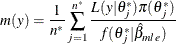
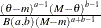
The parametric family for the auxiliary distribution is chosen to be Gaussian. The parameters that are subject to bounds are transformed accordingly
-
If
 , then
  .
.
-
If
 , then
  .
.
-
If
 , then
  .
.
-
If
 , then
  .
.
Assuming independence for the parameters that are subject to bounds, the auxiliary distribution to generate importance samples is
![\begin{equation*} \begin{pmatrix} \mb{p} \\ \mb{q} \\ \mb{r} \\ \mb{s} \end{pmatrix} \sim \mb{N} \left[ \begin{pmatrix} \mu _ p \\ \mu _{q} \\ \mu _{r} \\ \mu _{s} \\ \end{pmatrix}, \begin{pmatrix} \Sigma _ p & 0 & 0 & 0 \\ 0 & \Sigma _ q & 0 & 0 \\ 0 & 0 & \Sigma _ r & 0 \\ 0 & 0 & 0 & \Sigma _ r \\ \end{pmatrix} \right] \end{equation*}](images/etsug_countreg0417.png)
where  ,
,  ,
,  and
and  are vectors containing the transformations of the unbounded, bounded-below, bounded-above and bounded-above-and-below parameters.
Also, given the imposed independence structure,
are vectors containing the transformations of the unbounded, bounded-below, bounded-above and bounded-above-and-below parameters.
Also, given the imposed independence structure,  can be a non-diagonal matrix while
  ,
,  and
and  are imposed to be diagonal matrices.
Standard Distributions
Table 12.4 through Table 12.9 show all the distribution density functions that PROC COUNTREG recognizes. You specify these distribution densities in the PRIOR statement.
Table 12.4: Beta Distribution
|
PRIOR statement |
BETA(SHAPE1=a, SHAPE2=b, MIN=m, MAX=M) |
|
Note: Commonly |
|
|
Density |
|
|
Parameter restriction |
|
|
Range |
|
|
Mean |
|
|
Variance |
|
|
Mode |
|
|
Defaults |
SHAPE1=SHAPE2=1, |


![$ \left\{ \begin{array}{ll} \left[ m, M \right] & \mbox{when } a = 1, b = 1 \\ \left[ m, M \right) & \mbox{when } a = 1, b \neq 1 \\ \left( m, M \right] & \mbox{when } a \neq 1, b = 1 \\ \left( m, M \right) & \mbox{otherwise} \end{array} \right. $](images/etsug_countreg0432.png)
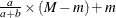
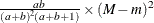
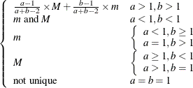


Table 12.5: Gamma Distribution
|
PRIOR statement |
GAMMA(SHAPE=a, SCALE=b ) |
|
Density |
|
|
Parameter restriction |
|
|
Range |
|
|
Mean |
|
|
Variance |
|
|
Mode |
|
|
Defaults |
SHAPE=SCALE=1 |
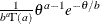


Table 12.6: Inverse Gamma Distribution
|
PRIOR statement |
IGAMMA(SHAPE=a, SCALE=b) |
|
Density |
|
|
Parameter restriction |
|
|
Range |
|
|
Mean |
|
|
Variance |
|
|
Mode |
|
|
Defaults |
SHAPE=2.000001, SCALE=1 |
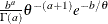


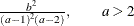

Table 12.7: Normal Distribution
|
PRIOR statement |
NORMAL(MEAN= |
|
Density |
|
|
Parameter restriction |
|
|
Range |
|
|
Mean |
|
|
Variance |
|
|
Mode |
|
|
Defaults |
MEAN=0, VAR=1000000 |


Table 12.8: t Distribution
|
PRIOR statement |
T(LOCATION= |
|
Density |
|
|
Parameter restriction |
|
|
Range |
|
|
Mean |
|
|
Variance |
|
|
Mode |
|
|
Defaults |
LOCATION=0, DF=3 |

![$\frac{\Gamma \left(\frac{\nu +1}{2}\right)}{\Gamma \left(\frac{\nu }{2}\right)\sqrt {\pi \nu }}\left[1+\frac{(\theta -\mu )^2}{\nu }\right]^{-\frac{\nu +1}{2}} $](images/etsug_countreg0453.png)


Table 12.9: Uniform Distribution
|
PRIOR statement |
UNIFORM(MIN=m, MAX=M) |
|
Density |
|
|
Parameter restriction |
|
|
Range |
|
|
Mean |
|
|
Variance |
|
|
Mode |
Not unique |
|
Defaults |
MIN |

![$ \theta \in [m, M]$](images/etsug_countreg0458.png)


