The COUNTREG Procedure
- Overview
- Getting Started
-
Syntax
 Functional SummaryPROC COUNTREG StatementBAYES StatementBOUNDS StatementBY StatementCLASS StatementDISPMODEL StatementFREQ StatementINIT StatementMODEL StatementNLOPTIONS StatementOUTPUT StatementPERFORMANCE StatementPRIOR StatementRESTRICT StatementSCORE StatementSHOW StatementSPATIALDISPEFFECTS StatementSPATIALEFFECTS StatementSPATIALID StatementSPATIALZEROEFFECTS StatementSTORE StatementTEST StatementWEIGHT StatementZEROMODEL Statement
 -
DetailsSpecification of RegressorsMissing ValuesPoisson RegressionConway-Maxwell-Poisson RegressionNegative Binomial RegressionZero-Inflated Count Regression OverviewZero-Inflated Poisson RegressionZero-Inflated Conway-Maxwell-Poisson RegressionZero-Inflated Negative Binomial RegressionSpatial Lag of X ModelVariable SelectionPanel Data AnalysisBY Groups and Scoring with an Item StoreParameter Naming Conventions for the RESTRICT, TEST, BOUNDS, and INIT StatementsComputational ResourcesNonlinear Optimization OptionsCovariance Matrix TypesDisplayed OutputBayesian AnalysisPrior DistributionsAutomated MCMC AlgorithmMarginal LikelihoodOUTPUT OUT= Data SetOUTEST= Data SetODS Table NamesODS Graphics
-
Examples
- References
Automated MCMC Algorithm
The main purpose of the automated MCMC algorithm is to provide the user with the opportunity to obtain a good approximation of the posterior distribution without initializing the MCMC algorithm: initial values, proposal distributions, burn-in, and number of samples.
The automated MCMC algorithm has two phases: tuning and sampling. The tuning phase has two main concerns: the choice of a good proposal distribution and the search for the stationary region of the posterior distribution. In the sampling phase, the algorithm decides how many samples are necessary to obtain good approximations of the posterior mean and some quantiles of interest.
Tuning Phase
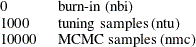
During the tuning phase, the algorithm tries to search for a good proposal distribution and, at the same time, to reach the stationary region of the posterior. The choice of the proposal distribution is based on the analysis of the acceptance rates. This is similar to what is done in PROC MCMC; for more information, see Chapter 73: The MCMC Procedure in SAS/STAT 14.1 User's Guide. For the stationarity analysis, the main idea is to run two tests, Geweke (Ge) and Heidleberger-Welch (HW), on the posterior chains at the end of each attempt. For more information, see Chapter 7: Introduction to Bayesian Analysis Procedures in SAS/STAT 14.1 User's Guide. If the stationarity hypothesis is rejected, then the number of tuning samples is increased and the tests are repeated in the next attempt. After 10 attempts, the tuning phase ends regardless of the results. The tuning parameters for the first attempt are fixed:
For the remaining attempts, the tuning parameters are adjusted dynamically. More specifically, each parameter is assigned an acceptance ratio (AR) of the stationarity hypothesis,
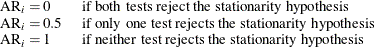
for  . Then, an overall stationarity average (SA) for all parameters ratios is evaluated,

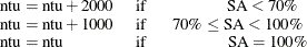
and the number of tuning samples is updated accordingly:
The Heidelberger-Welch test also provides an indication of how much burn-in should be used. The algorithm requires this burn-in
to be  . If that is not the case, the burn-in is updated accordingly,
 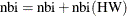 , and a new tuning attempt is made. This choice is motivated by the fact that the burn-in must be discarded in order to reach
the stationary region of the posterior distribution.
, and a new tuning attempt is made. This choice is motivated by the fact that the burn-in must be discarded in order to reach
the stationary region of the posterior distribution.
The number of samples that the Raftery-Lewis nmc(RL) diagnostic tool predicts is also considered:  . For more information, see Chapter 7: Introduction to Bayesian Analysis Procedures in SAS/STAT 14.1 User's Guide. However, in order to exit the tuning phase,
  is not required.
Sampling Phase
The main purpose of the sampling phase is to make sure that the mean and a quantile of interest are evaluated accurately. This can be tested by implementing the Heidelberger-Welch halfwidth test and by using the Raftery-Lewis diagnostic tool. In addition, the requirements that are defined in the tuning phase are also checked: the Geweke and Heidelberger-Welch tests must not reject the stationary hypothesis, and the burn-in that the Heidelberger-Welch test predicts must be zero.
The sampling phase has a maximum of 10 attempts. If the algorithm exceeds this limit, the sampling phase ends and indications
of how to improve sampling are given. The sampling phase first updates the burn-in with the information provided by the Heidelberger-Welch
test: . Then, it determines the difference between the actual number of samples and the number of samples that are predicted by
the Raftery-Lewis test: ![$\Delta [\text {nmc}(\text {RL})]=\text {nmc}(\text {RL})-\text {nmc}$](images/etsug_countreg0395.png) . The new number of samples is updated accordingly:
. The new number of samples is updated accordingly:
![\begin{equation*} \begin{tabular}{lll} $\text {nmc}=\text {nmc}+1000$ & if & \qquad \, \, \, $0<\Delta [\text {nmc}(\text {RL})]\leq 10000$ \\ $\text {nmc}=\text {nmc}+\Delta [\text {nmc}(\text {RL})]$ & if & \, \, \, $10000<\Delta [\text {nmc}(\text {RL})]\leq 300000$ \\ $\text {nmc}=\text {nmc}+300000$ & if & $300000<\Delta [\text {nmc}(\text {RL})]$ \end{tabular}\end{equation*}](images/etsug_countreg0396.png)
Finally, the Heidelberger-Welch halfwidth test checks whether the sample mean is accurate. If the mean of any parameters is not considered to be accurate, the number of samples is increased:
![\begin{equation*} \begin{tabular}{lll} $\text {nmc}=\text {nmc}+\{ 10000-\Delta [\text {nmc}(\text {RL})]\} $ & if & $10000-\Delta [\text {nmc}(\text {RL})]\geq 0$ \\ $\text {nmc}=\text {nmc}$ & if & $10000-\Delta [\text {nmc}(\text {RL})]<0$ \end{tabular}\end{equation*}](images/etsug_countreg0397.png)