The TPSPLINE Procedure

Example 116.2 Spline Model with Higher-Order Penalty

This example continues the analysis of the data set Measure to illustrate how you can use PROC TPSPLINE to fit a spline model with a higher-order penalty term. Spline models with high-order penalty terms move low-order polynomial terms into the polynomial space. Hence, there is no penalty for these terms, and they can vary without constraint.

As shown in the previous analyses, the final model for the data set Measure must include quadratic terms for both $x_1$ and $x_2$ . This example fits the following model:

$y = \beta _0 + \beta _1 x_1 + \beta _2 x_1^2 + \beta _3 x_2 + \beta _4 x_2^2 + \beta _5 x_1x_2 + f(x_1,x_2)$

The model includes quadratic terms for both variables, although it differs from the usual linear model. The nonparametric term $f(x_1,x_2)$ explains the variation of the data that is unaccounted for by a simple quadratic surface.

To modify the order of the derivative in the penalty term, specify the M= option. The following statements specify the option M=3 in order to include the quadratic terms in the polynomial space:

data Measure;
   set Measure;
   x1sq = x1*x1;
   x2sq = x2*x2;
   x1x2 = x1*x2;
run;

proc tpspline data= Measure;
   model y = (x1 x2) / m=3;
   score data = pred out = predy;
run;

Output 116.2.1 displays the results from these statements.

Output 116.2.1: Output from PROC TPSPLINE with M=3

The TPSPLINE Procedure

Dependent Variable: y

Summary of Input Data Set
Number of Non-Missing Observations	50
Number of Missing Observations	0
Unique Smoothing Design Points	25

Summary of Final Model
Number of Regression Variables	0
Number of Smoothing Variables	2
Order of Derivative in the Penalty	3
Dimension of Polynomial Space	6

Summary Statistics of Final Estimation
log10(n*Lambda)	-3.7831
Smoothing Penalty	2092.4495
Residual SS	0.2731
Tr(I-A)	29.1716
Model DF	20.8284
Standard Deviation	0.0968
GCV	0.0160

The model contains six terms in the polynomial space is the number of columns in ( $(\{ 1,x_1,x_1^2,x_1x_2,x_2,x_2^2\} )=6$ ). Compare Output 116.2.1 with Output 116.1.1: the $\log _{10}(n\lambda )$ value and the smoothing penalty differ significantly. In general, these terms are not directly comparable for different models. The final estimate based on this model is close to the estimate based on the model by using the default, M=2.

In the following statements, the REG procedure fits a quadratic surface model to the data set Measure:

proc reg data= Measure;
   model y = x1 x1sq x2 x2sq x1x2;
run;

The results are displayed in Output 116.2.2.

Output 116.2.2: Quadratic Surface Model: The REG Procedure

The REG Procedure

Model: MODEL1

Dependent Variable: y

Analysis of Variance
Source	DF	Sum of Squares	Mean Square	F Value	Pr > F
Model	5	443.20502	88.64100	436.33	<.0001
Error	44	8.93874	0.20315
Corrected Total	49	452.14376

Root MSE	0.45073	R-Square	0.9802
Dependent Mean	15.08548	Adj R-Sq	0.9780
Coeff Var	2.98781

Parameter Estimates
Variable	DF	Parameter Estimate	Standard Error	t Value	Pr > \|t\|
Intercept	1	14.90834	0.12519	119.09	<.0001
x1	1	0.01292	0.09015	0.14	0.8867
x1sq	1	-4.85194	0.15237	-31.84	<.0001
x2	1	0.02618	0.09015	0.29	0.7729
x2sq	1	5.20624	0.15237	34.17	<.0001
x1x2	1	-0.04814	0.12748	-0.38	0.7076

The REG procedure produces slightly different results. To fit a similar model with PROC TPSPLINE, you can use a MODEL statement that specifies the degrees of freedom with the DF= option. You can also use a large value for the LOGNLAMBDA0= option to force a parametric model fit.

Because there is one degree of freedom for each of the terms intercept, x1, x2, x1sq, x2sq, and x1x2, the DF=6 option is used as follows:

proc tpspline data=measure;
   model  y=(x1 x2) /m=3 df=6 lognlambda=(-4 to 1 by 0.5);
   score data = pred
          out = predy;
run;

The fit statistics are displayed in Output 116.2.3.

Output 116.2.3: Output from PROC TPSPLINE Using M=3 and DF=6

The TPSPLINE Procedure

Dependent Variable: y

Summary of Final Model
Number of Regression Variables	0
Number of Smoothing Variables	2
Order of Derivative in the Penalty	3
Dimension of Polynomial Space	6

GCV Function
log10(n*Lambda)	GCV
-4.000000	0.016330	*
-3.500000	0.016889
-3.000000	0.027496
-2.500000	0.067672
-2.000000	0.139642
-1.500000	0.195727
-1.000000	0.219512
-0.500000	0.227306
0	0.229740
0.500000	0.230504
1.000000	0.230745

Note: * indicates minimum GCV value.

Summary Statistics of Final Estimation
log10(n*Lambda)	2.3830
Smoothing Penalty	0.0000
Residual SS	8.9384
Tr(I-A)	43.9997
Model DF	6.0003
Standard Deviation	0.4507
GCV	0.2309

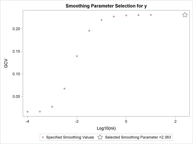
Output 116.2.4 shows the GCV values for the list of supplied $\log _{10}(n\lambda )$ values in addition to the fitted model with fixed degrees of freedom 6. The fitted model has a larger GCV value than all other examined models.

Output 116.2.4: Criterion Plot

The final estimate is based on 6.000330 degrees of freedom because there are already 6 degrees of freedom in the polynomial space and the search range for $\lambda$ is not large enough (in this case, setting DF=6 is equivalent to setting $\lambda = \infty$ ).

The standard deviation and RSS (Output 116.2.3) are close to the sum of squares for the error term and the root MSE from the linear regression model (Output 116.2.2), respectively.

For this model, the optimal $\log _{10}(n\lambda )$ is around –3.8, which produces a standard deviation estimate of 0.096765 (see Output 116.2.1) and a GCV value of 0.016051, while the model that specifies DF=6 results in a $\log _{10}(n\lambda )$ larger than 1 and a GCV value larger than 0.23074. The nonparametric model, based on the GCV, should provide better prediction, but the linear regression model can be more easily interpreted.