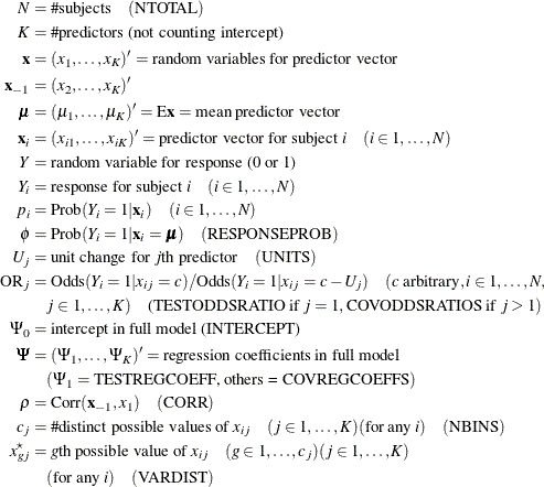
The POWER Procedure
- Overview
-
Getting Started

-
SyntaxPROC POWER StatementCOXREG StatementLOGISTIC StatementMULTREG StatementONECORR StatementONESAMPLEFREQ StatementONESAMPLEMEANS StatementONEWAYANOVA StatementPAIREDFREQ StatementPAIREDMEANS StatementPLOT StatementTWOSAMPLEFREQ StatementTWOSAMPLEMEANS StatementTWOSAMPLESURVIVAL StatementTWOSAMPLEWILCOXON Statement
-
Details
-
ExamplesOne-Way ANOVAThe Sawtooth Power Function in Proportion AnalysesSimple AB/BA Crossover DesignsNoninferiority Test with Lognormal DataMultiple Regression and CorrelationComparing Two Survival CurvesConfidence Interval PrecisionCustomizing PlotsBinary Logistic Regression with Independent PredictorsWilcoxon-Mann-Whitney Test
- References
Analyses in the LOGISTIC Statement
Likelihood Ratio Chi-Square Test for One Predictor (TEST=LRCHI)
The power-computing formula is based on Shieh and O’Brien (1998); Shieh (2000); Self, Mauritsen, and Ohara (1992), and Hsieh (1989).
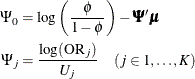
Define the following notation for a logistic regression analysis:
The logistic regression model is
![\[ \log \left( \frac{p_ i}{1-p_ i} \right) = \Psi _0 + \bPsi ’\mb{x}_ i \]](images/statug_power0095.png)
The hypothesis test of the first predictor variable is

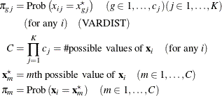
Assuming independence among all predictor variables,  is defined as follows:
![\[ \pi _ m = \prod _{j=1}^{K} \pi _{h(m,j) j} \quad (m \in 1, \ldots , C) \]](images/statug_power0098.png)
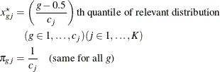
where  is calculated according to the following algorithm:
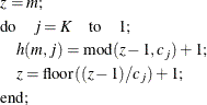
This algorithm causes the elements of the transposed vector 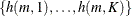 to vary fastest to slowest from right to left as m increases, as shown in the following table of values:
![\[ \begin{array}{cc|ccccc}& & & & j & & \\ h(m,j) & & 1 & 2 & \cdots & K-1 & K \\ \hline & 1 & 1 & 1 & \cdots & 1 & 1 \\ & 1 & 1 & 1 & \cdots & 1 & 2 \\ & \vdots & & & \vdots & & \\ & \vdots & 1 & 1 & \cdots & 1 & c_ K \\ & \vdots & 1 & 1 & \cdots & 2 & 1 \\ & \vdots & 1 & 1 & \cdots & 2 & 2 \\ & \vdots & & & \vdots & & \\ m & \vdots & 1 & 1 & \cdots & 2 & c_ K \\ & \vdots & & & \vdots & & \\ & \vdots & c_1 & c_2 & \cdots & c_{K-1} & 1 \\ & \vdots & c_1 & c_2 & \cdots & c_{K-1} & 2 \\ & \vdots & & & \vdots & & \\ & C & c_1 & c_2 & \cdots & c_{K-1} & c_ K \\ \end{array} \]](images/statug_power0102.png)
The  values are determined in a completely analogous manner.
The discretization is handled as follows (unless the distribution is ordinal, or binomial with sample size parameter at least
as large as requested number of bins): for  , generate
  quantiles at evenly spaced probability values such that each such quantile is at the midpoint of a bin with probability
  . In other words,
The primary noncentrality for the power computation is
![\[ \Delta ^\star = 2 \sum _{m=1}^ C \pi _ m \left[ b’(\theta _ m) \left(\theta _ m - \theta ^\star _ m \right) - \left( b(\theta _ m) - b(\theta ^\star _ m) \right) \right] \]](images/statug_power0108.png)
where
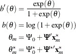
where

The power is
![\[ \mr{power} = P\left(\chi ^2(1, \Delta ^\star N (1-\rho ^2)) \ge \chi ^2_{1-\alpha }(1)\right) \]](images/statug_power0111.png)
The factor  is the adjustment for correlation between the predictor that is being tested and other predictors, from Hsieh (1989).
Alternative input parameterizations are handled by the following transformations: