The POWER Procedure

Analyses in the COXREG Statement

Score Test of a Single Scalar Predictor in Cox Proportional Hazards Regression (TEST=SCORE)

The power-computing formula is based on Hsieh and Lavori (2000, equation (2) and the section "Variance Inflation Factor" on page 556).

Define the following notation for a Cox proportional hazards regression analysis:

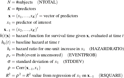
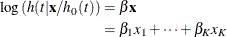
$\begin{align*} N & = \# \text {subjects}\quad (\text {NTOTAL}) \\ K & = \# \text {predictors} \\ \mb{x} & = (x_{1}, \ldots , x_{K})’ = \text {vector of predictors} \\ x_1 & = \text {predictor of interest} \\ \mb{x}_{-1} & = (x_{2}, \ldots , x_{K})’ \\ h(t|\mb{x}) & = \text {hazard function for survival time given $\mb{x}$, evaluated at time \Mathtext{t}} \\ h_0(t) & = \text {baseline hazard at time \Mathtext{t}} \\ h_\mr {r} & = \text {hazard ratio for one-unit increase in $x_1$} \quad \text {(HAZARDRATIO)} \\ p_ e & = \mr{Prob} (\text {event is uncensored}) \quad (\text {EVENTPROB}) \\ \sigma & = \text {standard deviation of $x_1$} \quad \text {(STDDEV)} \\ \rho & = \mr{Corr}(\mb{x}_{-1}, x_1) \\ R^2 & = \rho ^2 = \text {$R^2$ value from regression of $x_1$ on $\mb{x}_{-1}$} \quad (\text {RSQUARE}) \\ \end{align*}$

The Cox proportional hazards regression model is

$\begin{align*} \log \left( h(t|\mb{x} / h_0(t) \right) & = \beta \mb{x} \\ & = \beta _1 x_1 + \cdots + \beta _ K x_ K \\ \end{align*}$

You can convert a regression coefficient to a hazard ratio by using the equation $h_\mr {r} = \exp (\beta _1)$ .

The hypothesis test of the first predictor variable is

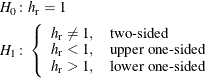
$\begin{align*} H_{0}\colon & h_\mr {r}=1 \\ H_{1}\colon & \left\{ \begin{array}{ll} h_\mr {r} \ne 1, & \mbox{two-sided} \\ h_\mr {r} < 1, & \mbox{upper one-sided} \\ h_\mr {r} > 1, & \mbox{lower one-sided} \\ \end{array} \right. \\ \end{align*}$

The upper and lower one-sided cases are expressed differently than in other analyses. This is because $h_\mr {r} > 1$ corresponds to a negative correlation between the tested predictor and survival and thus, by the convention used in PROC POWER for regression analyses, the lower side.

The approximate power is

$\mr{power} = \left\{ \begin{array}{ll} \Phi \left( z_\alpha - \sigma \sqrt {N p_ e (1 - R^2)} \log (h_\mr {r}) \right), & \mbox{upper one-sided} \\ 1 - \Phi \left( z_{1-\alpha } - \sigma \sqrt {N p_ e (1 - R^2)} \log (h_\mr {r}) \right), & \mbox{lower one-sided} \\ \Phi \left( z_\frac {\alpha }{2} - \sigma \sqrt {N p_ e (1 - R^2)} \log (h_\mr {r}) \right) + 1 - \Phi \left( z_{1-\frac{\alpha }{2}} - \sigma \sqrt {N p_ e (1 - R^2)} \log (h_\mr {r}) \right), & \mbox{two-sided} \\ \end{array} \right. \\$

For the one-sided cases, a closed-form inversion of the power equation yields an approximate total sample size

$N = \left( \frac{\left( z_{\mr{power}} + z_{1-\alpha } \right)^2}{p_ e (1-R^2) \sigma ^2 \log (h_\mr {r})} \right)$

For the two-sided case, the solution for N is obtained by numerically inverting the power equation.