The NLIN Procedure
- Overview
-
Getting Started

-
Syntax
-
DetailsAutomatic DerivativesMeasures of Nonlinearity, Diagnostics and InferenceMissing ValuesSpecial VariablesTroubleshootingComputational MethodsOutput Data SetsConfidence IntervalsCovariance Matrix of Parameter EstimatesConvergence MeasuresDisplayed OutputIncompatibilities with SAS 6.11 and Earlier Versions of PROC NLINODS Table NamesODS Graphics
-
Examples
- References
Measures of Nonlinearity, Diagnostics and Inference
- Box’s Measure of Bias
- Hougaard’s Measure of Skewness
- Relative Curvature Measures of Nonlinearity
- Leverage in Nonlinear Regression
- Local Influence in Nonlinear Regression
- Residuals in Nonlinear Regression
- Profiling Parameters and Assessing the Influence of Observations on Parameter Estimates
- Bootstrap Resampling and Estimation
A "close-to-linear" nonlinear regression model, in the sense of Ratkowsky (1983, 1990), is a model in which parameter estimators have properties similar to those in a linear regression model. That is, the least squares estimators of the parameters are close to being unbiased and normally distributed, and they have minimum variance.
A nonlinear regression model sometimes fails to be close to linear due to the properties of one or several parameters. When this occurs, bias in the parameter estimates can render inferences that use the reported standard errors and confidence limits invalid.
PROC NLIN provides various measures of nonlinearity. To assess the nonlinearity of a model-data combination, you can use both of the following complementary sets of measures:
Furthermore, PROC NLIN provides residual, leverage, and local-influence diagnostics (St. Laurent and Cook 1993).
In the following several sections, these nonlinearity measures and diagnostics are discussed. For this material, several basic
definitions are required. Let  be the Jacobian matrix for the model,
  , and let
  and
and  be the components of the QR decomposition of
  of , where is an
  orthogonal matrix. Finally, let
  be the inverse of the matrix constructed from the first p rows of the
  dimensional matrix (that is,
  ). Next define
![\begin{align*} \left[\mb{H}_ j\right]_{kl} & = \frac{\partial ^2 \mb{f}_ j}{\partial \bbeta _ k \partial \bbeta _ l}\\ \left[\mb{U}_ j\right]_{kl} & = \sum _{mn} \mb{B}’_{km} \left[\mb{H}_ j\right]_{mn} \mb{B}_{nl} \\ \left[\mb{A}_ j\right]_{kl} & = \sqrt {p \times \mr{mse} }\sum _{m} \mb{Q}’_{jm} \left[\mb{U}_ m\right]_{kl}\, , \end{align*}](images/statug_nlin0082.png)
where  ,
,  and the acceleration array
  are three-dimensional
  matrices. The first p faces of the acceleration array constitute a
  parameter-effects array and the last
  faces constitute the
  intrinsic curvature array (Bates and Watts 1980). The previous and subsequent quantities are computed at the least squares parameter estimators.
Box’s Measure of Bias
The degree to which parameter estimators exhibit close-to-linear behavior can be assessed with Box’s bias (Box 1971) and Hougaard’s measure of skewness (Hougaard 1982, 1985). The bias and percentage bias measures are available through the BIAS option in the PROC NLIN statement. Box’s bias measure is defined as
![\begin{align*} \widehat{\mr{E}}\left[ \widehat{\beta } - \beta \right] & = -\frac{\sigma ^2}{2} \left(\mb{X}’ \bW \mb{X}\right)^{-1} \sum ^{n}_{i=1} w_ i \mb{x}’_ i \, \text {Tr}\left( \left(\mb{X}’ \bW \mb{X}\right)^{-1} \left[\mb{H}_{i}\right]\right) \end{align*}](images/statug_nlin0090.png)
where  if the SIGSQ
option is not set. Otherwise,
if the SIGSQ
option is not set. Otherwise,  is the value you set with the SIGSQ
option.
is the value you set with the SIGSQ
option.  is the diagonal weight matrix specified with the
 _WEIGHT_ variable (or the identity matrix if _WEIGHT_ is not defined) and ![$\left[\mb{H}_{i}\right]$](images/statug_nlin0092.png) is the
is the  Hessian matrix at the ith observation. In the case of unweighted least squares, the bias formula can be expressed in terms of the acceleration array
,
Hessian matrix at the ith observation. In the case of unweighted least squares, the bias formula can be expressed in terms of the acceleration array
,
![\begin{align*} \widehat{\mr{E}}\left[ \widehat{\beta }_ i - {\beta }_ i\right] & = - \frac{\sigma ^2}{2 p \times \hbox{mse}} \sum ^{p}_{j,\, k=1} \mb{B}_{ij} \left[\mb{A}_ j\right]_{kk} \end{align*}](images/statug_nlin0094.png)
As the preceding formulas illustrate, the bias depends solely on the parameter-effects array, thereby permitting its reduction through reparameterization. Example 81.4 shows how changing the parameterization of a four-parameter logistic model can reduce the bias. Ratkowsky (1983, p. 21) recommends that you consider reparameterization if the percentage bias exceeds 1%.
Hougaard’s Measure of Skewness
In addition to Box’s bias, Hougaard’s measure of skewness,  (Hougaard 1982, 1985), is also provided in PROC NLIN to assess the close-to-linear behavior of parameter estimators. This measure is available
through the HOUGAARD
option in the PROC NLIN
statement. Hougaard’s skewness measure for the ith parameter is based on the third central moment, defined as
(Hougaard 1982, 1985), is also provided in PROC NLIN to assess the close-to-linear behavior of parameter estimators. This measure is available
through the HOUGAARD
option in the PROC NLIN
statement. Hougaard’s skewness measure for the ith parameter is based on the third central moment, defined as
![\[ \mr{E} \left[ \widehat{\beta }_ i - \mr{E}\left(\widehat{\beta }_ i\right)\right]^3 = - \left(\sigma ^2\right)^2 \sum _{jkl} [\mb{L}]_{ij}[\mb{L}]_{ik}[\mb{L}]_{il} \left( \left[\mb{V}_ j\right]_{kl}+[\mb{V}_ k]_{jl}+[\mb{V}_ l]_{jk}\right) \]](images/statug_nlin0096.png)
where the sum is a triple sum over the number of parameters and
![\[ \mb{L} = \left(\mb{X}’\mb{X}\right)^{-1} = \left( \frac{\partial \mb{f}}{\partial \bbeta ^\prime } \frac{\partial \mb{f}}{\partial \bbeta } \right)^{-1} \]](images/statug_nlin0097.png)
The term ![$[\mb{L}]_{ij}$](images/statug_nlin0098.png) denotes the value in row i, column j of the matrix
denotes the value in row i, column j of the matrix  . (Hougaard (1985) uses superscript notation to denote elements in this inverse.) The matrix
  is a three-dimensional array
![\begin{align*} \left[\mb{V}_ j\right]_{kl} & = \sum _{m=1}^ n \frac{\partial F_ m}{\partial \beta _ j} \frac{\partial ^2 F_ m}{\partial \beta _ k \partial \beta _ l} \end{align*}](images/statug_nlin0101.png)
The third central moment is then normalized using the standard error as
![\[ G_{1i} = \mr{E}\left[ \widehat{\beta }_ i - \mr{E}(\widehat{\beta }_ i)\right]^3 / \left(\sigma ^2 \times \left[ \mb{L} \right]_{ii} \right)^{3/2} \]](images/statug_nlin0102.png)
The previous expressions depend on the unknown values of the parameters and on the residual variance . In order to evaluate the Hougaard measure in a particular data set, the NLIN procedure computes
![\begin{align*} g_{1i} & = \widehat{\mr{E}}\left[ \widehat{\beta }_ i - \mr{E}(\widehat{\beta }_ i)\right]^3 /\left( \mr{mse} \times [\widehat{\mb{L}}]_{ii} \right) ^{3/2} \\ \widehat{\mr{E}}\left[ \widehat{\beta }_ i - \mr{E}(\widehat{\beta }_ i)\right]^3 & = - \mr{mse}^2 \sum _{jkl} [\widehat{\mb{L}}]_{ij} [\widehat{\mb{L}}]_{ik} [\widehat{\mb{L}}]_{il} \left( [\widehat{\mb{V}}_ j]_{kl} + [\widehat{\mb{V}}_ k]_{jl} + [\widehat{\mb{V}}_ l]_{jk} \right) \end{align*}](images/statug_nlin0103.png)
Following Ratkowsky (1990, p. 28), the parameter  is considered to be very close to linear, reasonably close, skewed, or quite nonlinear according to the absolute value of
the Hougaard measure
is considered to be very close to linear, reasonably close, skewed, or quite nonlinear according to the absolute value of
the Hougaard measure  being less than 0.1, between 0.1 and 0.25, between 0.25 and 1, or greater than 1, respectively.
Relative Curvature Measures of Nonlinearity
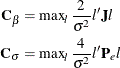
Bates and Watts (1980) formulated the maximum parameter-effects and maximum intrinsic curvature measures of nonlinearity to assess the close-to-linear behavior of nonlinear models. Ratkowsky (1990) notes that of the two curvature components in a nonlinear model, the parameter-effects curvature is typically larger. It is this component that you can affect by changing the parameterization of a model. PROC NLIN provides these two measures of curvature both through the STATS plot-option and through the NLINMEASURES option in the PROC NLIN statement.
The maximum parameter-effects and intrinsic curvatures are defined, in a compact form, as
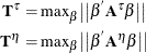
where  and
and  denote the maximum parameter-effects and intrinsic curvatures, while
  and
and  stand for the parameter-effects and intrinsic curvature arrays. The maximization is carried out over a unit-vector of the
parameter values (Bates and Watts 1980). In line with Bates and Watts (1980), PROC NLIN takes
stand for the parameter-effects and intrinsic curvature arrays. The maximization is carried out over a unit-vector of the
parameter values (Bates and Watts 1980). In line with Bates and Watts (1980), PROC NLIN takes  as the convergence tolerance for the maximum intrinsic and parameter-effects curvatures. Note that the preceding matrix products
involve contraction of the faces of the three-dimensional acceleration arrays with the normalized parameter vector,
as the convergence tolerance for the maximum intrinsic and parameter-effects curvatures. Note that the preceding matrix products
involve contraction of the faces of the three-dimensional acceleration arrays with the normalized parameter vector,  . The corresponding expressions for the RMS (root mean square) parameter-effects and intrinsic curvatures can be found in
Bates and Watts (1980).
. The corresponding expressions for the RMS (root mean square) parameter-effects and intrinsic curvatures can be found in
Bates and Watts (1980).
The statistical significance of and and the corresponding RMS values can be assessed by comparing these values with  , where F is the upper
  quantile of an F distribution with p and
  degrees of freedom (Bates and Watts 1980).
One motivation for fitting a nonlinear model in a different parameterization is to obtain a particular interpretation and to give parameter estimators more close-to-linear behavior. Example 81.4 shows how changing the parameterization of a four-parameter logistic model can reduce the parameter-effects curvature and can yield a useful parameter interpretation at the same time. In addition, Example 81.6 shows a nonlinear model with a high intrinsic curvature and the corresponding diagnostics.
Leverage in Nonlinear Regression
In contrast to linear regression, there are several measures of leverage in nonlinear regression. Furthermore, in nonlinear regression, the effect of a change in the ith response on the ith predicted value might depend on both the size of the change and the ith response itself (St. Laurent and Cook 1992). As a result, some observations might show superleverage —namely, leverages in excess of one (St. Laurent and Cook 1992).
PROC NLIN provides two measures of leverages: tangential and Jacobian leverages through the PLOTS
option in the PROC NLIN
statement and the H=
and J=
options of OUTPUT
statement. Tangential leverage,  , is based on approximating the nonlinear model with a linear model that parameterizes the tangent plane at the least squares
parameter estimators. In contrast, Jacobian leverage,
, is based on approximating the nonlinear model with a linear model that parameterizes the tangent plane at the least squares
parameter estimators. In contrast, Jacobian leverage,  , is simply defined as the instantaneous rate of change in the ith predicted value with respect to the ith response (St. Laurent and Cook 1992).
The mathematical formulas for tangential and Jacobian leverages are
![\begin{align*} \mb{H}_ i & = w_ i \mb{x}_ i(\mb{X}^{\prime }\mb{WX})^{-1} \mb{x}_ i^{\prime }\\ \mb{J}_ i & = w_ i \mb{x}_ i (\mb{X}^{\prime }\mb{WX}-[\mb{W\, e}][\mb{H}])^{-1} \mb{x}_ i^{\prime }\, , \end{align*}](images/statug_nlin0115.png)
where  is the vector of residuals, is the diagonal weight matrix if you specify the special variable
 _WEIGHT_ and otherwise the identity matrix, and i indexes the corresponding quantities for the ith observation. The brackets ![$[.][.]$](images/statug_nlin0117.png) indicate column multiplication as defined in Bates and Watts (1980). The preceding formula for tangential leverage holds if the gradient, Marquardt, or Gauss methods are used. For the Newton
method, the tangential leverage is set equal to the Jacobian leverage.
indicate column multiplication as defined in Bates and Watts (1980). The preceding formula for tangential leverage holds if the gradient, Marquardt, or Gauss methods are used. For the Newton
method, the tangential leverage is set equal to the Jacobian leverage.
In a model with a large intrinsic curvature, the Jacobian and tangential leverages can be very different. In fact, the two
leverages are identical only if the model provides an exact fit to the data ( ) or the model is intrinsically linear (St. Laurent and Cook 1993). This is also illustrated by the leverage plot and nonlinearity measures provided in Example 81.6.
Local Influence in Nonlinear Regression
St. Laurent and Cook (1993) suggest using  , the direction that yields the maximum normal curvature, to assess the local influence of an additive perturbation to the
response variable on the estimation of the parameters and variance of a nonlinear model. Defining the normal curvature components
, the direction that yields the maximum normal curvature, to assess the local influence of an additive perturbation to the
response variable on the estimation of the parameters and variance of a nonlinear model. Defining the normal curvature components
where  is the Jacobian leverage matrix and
  , you choose the that results in the maximum of the two curvature components (St. Laurent and Cook 1993). PROC NLIN provides through the PLOTS
option in the PROC NLIN
statement and the LMAX=
option in the OUTPUT
statement. Example 81.6 shows a plot of for a model with high intrinsic curvature.
, you choose the that results in the maximum of the two curvature components (St. Laurent and Cook 1993). PROC NLIN provides through the PLOTS
option in the PROC NLIN
statement and the LMAX=
option in the OUTPUT
statement. Example 81.6 shows a plot of for a model with high intrinsic curvature.
Residuals in Nonlinear Regression
If a nonlinear model is intrinsically nonlinear, using the residuals  for diagnostics can be misleading (Cook and Tsai 1985). This is due to the fact that in correctly specified intrinsically nonlinear models, the residuals have nonzero means and
different variances, even when the original error terms have identical variances. Furthermore, the covariance between the
residuals and the predicted values tends to be negative semidefinite, complicating the interpretation of plots based on (Cook and Tsai 1985).
for diagnostics can be misleading (Cook and Tsai 1985). This is due to the fact that in correctly specified intrinsically nonlinear models, the residuals have nonzero means and
different variances, even when the original error terms have identical variances. Furthermore, the covariance between the
residuals and the predicted values tends to be negative semidefinite, complicating the interpretation of plots based on (Cook and Tsai 1985).
Projected residuals are proposed by Cook and Tsai (1985) to overcome these shortcomings of residuals, which are henceforth called raw (ordinary) residuals to differentiate them from their projected counterparts. Projected residuals have zero means and are uncorrelated with the predicted values. In fact, projected residuals are identical to the raw residuals in intrinsically linear models.
PROC NLIN provides raw and projected residuals, along with their standardized forms. In addition, the mean or expectation of the raw residuals is available. These can be accessed with the PLOTS option in the PROC NLIN statement and the OUTPUT statement options PROJRES= , PROJSTUDENT= , RESEXPEC= , RESIDUAL= and STUDENT= .
Denote the projected residuals by  and the expectation of the raw residuals by
 ![$\mr{E}[\mb{e}]$](images/statug_nlin0125.png) . Then
. Then
![\begin{align*} \mb{e}_{p} & = \left(\mb{I}_ n - \mb{P}_{xh}\right)\mb{e}\, \\ \mr{E} \left[\mb{e}_ i\right] & = -\frac{\sigma ^2}{2}\, \sum ^{n}_{j=1} \tilde{\mb{P}}_{x,\, ij} \text {Tr}\left(\, \left[\mb{H}_ j\right] \, \left(\mb{X}’\mb{X}\right)^{-1}\, \right) \end{align*}](images/statug_nlin0126.png)
where  is the ith observation raw residual,
  is an n-dimensional identity matrix,
  is the projector onto the column space of
  , and
, and  . The preceding formulas are general with the projectors defined accordingly to take the weighting into consideration. In
unweighted least squares,
. The preceding formulas are general with the projectors defined accordingly to take the weighting into consideration. In
unweighted least squares, ![$\mr{E} \left[\mb{e}\right]$](images/statug_nlin0132.png) reduces to
reduces to
![\begin{align*} \mr{E} \left[\mb{e}\right] & = -\frac{1}{2} \sigma ^2 \tilde{\mb{Q}}\, \mb{a}\, \end{align*}](images/statug_nlin0133.png)
with  being the last columns of the matrix in the QR decomposition of and the dimensional vector
  being defined in terms of the intrinsic acceleration array
![\begin{align*} \mb{a}_ i & = \sum ^{p}_{j=1}\left[\mb{A}_{i+p}\right]_{jj} \end{align*}](images/statug_nlin0136.png)
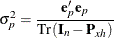
Standardization of the projected residuals requires the variance of the projected residuals. This is estimated using the formula (Cook and Tsai 1985)
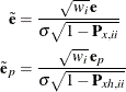
The standardized raw and projected residuals, denoted by  and
and  respectively, are given by
The use of raw and projected residuals for diagnostics in nonlinear regression is illustrated in Example 81.6.
Profiling Parameters and Assessing the Influence of Observations on Parameter Estimates
The global measures of nonlinearity, discussed in the preceding section, are very useful for assessing the overall nonlinearity of the model. However, the impact of global nonlinearity on inference regarding subsets of the parameter set cannot be easily determined (Cook and Tsai 1985). The impact of the nonlinearity on the uncertainty of individual parameters can be efficiently described by profile t plots and confidence curves (Bates and Watts 1988; Cook and Weisberg 1990).
A profile t plot for parameter is a plot of the likelihood ratio pivotal statistic,  , and the corresponding Wald pivotal statistic,
  (Bates and Watts 1988). The likelihood ratio pivotal statistic is defined as
![\[ \tau (\beta ) = \mbox{sign}(\beta - \hat{\beta })\, \mbox{L}(\beta ) \]](images/statug_nlin0143.png)
with
![\[ \mbox{L}(\beta ) = \left( \frac{\mbox{SSE}(\beta , \tilde{\Theta }) - \mbox{SSE}(\hat{\beta }, \hat{\Theta }) }{\mbox{mse}} \right)^{1/2} \]](images/statug_nlin0144.png)
where is the profile parameter and  refers to the remaining parameters.
  is the sum of square errors where the profile parameter is constrained at a given value and
  is the least squares estimate of conditional on a given value of . In contrast,
  is the sum of square errors for the full model. For linear models, matches , which is defined as
![\[ \sigma (\beta ) = \frac{\beta - \hat{\beta }}{\mbox{stderr}_\beta } \]](images/statug_nlin0149.png)
where is the constrained value,  is the estimated value for the parameter, and
  is the standard error for the parameter. Usually a profile t plot is overlaid with a reference line that passes through the origin and has a slope of one. PROC NLIN follows this convention.
A confidence curve for a particular parameter is useful for validating Wald-based confidence intervals for the parameter against
likelihood-based confidence intervals (Cook and Weisberg 1990). A confidence curve contains a scatter plot of the constrained parameter value versus  . The Wald-based confidence intervals are overlaid as two straight lines that pass through
  with a slope of
  . Hence, for different levels of significance, you can easily compare the Wald-based confidence intervals against the corresponding
confidence intervals that are based on the likelihood ratio. Cook and Weisberg (1990) recommend that you report a single Wald-based confidence interval only if there is a good agreement between the Wald and
likelihood intervals up to at least the 99% confidence level.
. Hence, for different levels of significance, you can easily compare the Wald-based confidence intervals against the corresponding
confidence intervals that are based on the likelihood ratio. Cook and Weisberg (1990) recommend that you report a single Wald-based confidence interval only if there is a good agreement between the Wald and
likelihood intervals up to at least the 99% confidence level.
Compared to local influence, the leave-one-out method performs a more complete analysis of the influence of observations on the values of parameter estimates. In this method, jackknife resampling removes each observation in turn and fits the model to the remaining data set. Hence, a data set with n observations will have n corresponding data sets with n–1 observations. The impact of each observation on a parameter is assessed by the absolute relative percentage change in the value of the parameter compared with the reference value from the full data.
Bootstrap Resampling and Estimation
Bootstrap resampling and estimation methods can be used to produce confidence intervals and covariance matrix estimates that
have second-order,  accuracy, where n is the number of observations (DiCiccio and Efron 1996). In contrast, the standard Wald-based confidence interval has first-order,
  accuracy. Bootstrap methods achieve this higher accuracy at the cost of an orders-of-magnitude increase in numerical computation
compared to standard asymptotic approximations. However, dramatic increases in performance and decreases in the cost of numerical
computation have made bootstrap methods very attractive for routine statistical inference (MacKinnon 2002).
accuracy. Bootstrap methods achieve this higher accuracy at the cost of an orders-of-magnitude increase in numerical computation
compared to standard asymptotic approximations. However, dramatic increases in performance and decreases in the cost of numerical
computation have made bootstrap methods very attractive for routine statistical inference (MacKinnon 2002).
PROC NLIN samples as many bootstrap sample data sets (replicates) as you specify in the NSAMPLES= option and performs least squares fit on each replicate. For each least squares fit, PROC NLIN uses the original parameter estimates as starting values for the model parameters. The statistics from the least squares fits that converge are collected and used to produce confidence intervals, covariance and correlation matrices, and histograms and scatter plots of the bootstrap parameter estimates.
Each replicate is obtained by sampling the residuals instead of the input data set. The sampled residuals are used to simulate the response by using a bootstrap data generating process (DGP). PROC NLIN’s bootstrap DGP produces replicates that contain the same number of observations as the number of usable observations in the input data set. In fact, the bootstrap DGP for a particular replicate starts by discarding the input data set observations that PROC NLIN deems unusable during the original least squares estimation. The next step of the bootstrap DGP for a replicate can be represented by the formula
![\[ \tilde{Y}_ i = f(\hat{\bbeta }; \mb{z}_{i}^\prime ) + \tilde{\epsilon }_ i \]](images/statug_nlin0156.png)
where  is the ith simulated response,
  is the original least squares parameter estimate,
  is the ith regressor vector, and
  is the ith simulated error.
PROC NLIN makes several bootstrap DGP types available in the DGP=
option of the BOOTSTRAP
statement. These bootstrap DGP types differ only in how they obtain the ith simulated error, . In general, can be represented as
![\[ \tilde{\epsilon }_ i = {\mb{s}}_ r {\hat{\mb{e}}}_{r} \]](images/statug_nlin0161.png)
where r is a uniform random integer between 1 and the number of usable observations,  is a scale factor that depends on the chosen bootstrap DGP options, and
  is the rth residual obtained from the rth usable observation of the original least squares fit. The scale factor, , that captures the differences among the various bootstrap DGP types takes one of the following values:
![\[ \mb{s}_ r = \left\{ \begin{array}{ll} 1 & \quad \text {if DGP=RESIDUAL(RAW)} \cr \sqrt {\frac{\mb{n}}{\mb{n} - \mb{p}}} & \quad \text {if DGP=RESIDUAL(ADJSSE)} \cr \frac{1}{\sqrt {1 - \mb{H}_ r}} & \quad \text {if DGP=RESIDUAL(TAN)} \cr \frac{1}{\sqrt {1 - \mb{J}_ r}} & \quad \text {if DGP=RESIDUAL(JAC)} \cr \frac{\gamma }{\sqrt {1 - \mb{H}_ r}} & \quad \text {if DGP=WILD} \end{array} \right. \]](images/statug_nlin0164.png)
In the preceding formula,  is the number of usable observations,
  is the number of model parameters, and
  and
and  are the rth tangential and Jacobian leverages, respectively. For the WILD bootstrap DGP (Wu 1986), which is the only bootstrap DGP type exclusively available for weighted least squares,
  is a random number given by
![\[ \gamma = \left\{ \begin{array}{ll} -\frac{\sqrt {5} - 1}{2} & \, \, \, \mr{with}\, \, \mr{probability} \, \, \, \, \, \frac{\sqrt {5} + 1}{2\sqrt {5}} \cr \frac{\sqrt {5} + 1}{2} & \, \, \, \mr{with}\, \, \, \mr{ probability} \, \, \, \, \, \frac{\sqrt {5} - 1}{2\sqrt {5}} \end{array} \right. \]](images/statug_nlin0170.png)
PROC NLIN makes three types of bootstrap confidence intervals available in the BOOTCI
option in the BOOTSTRAP
statement. These confidence intervals are the percentile, normal, and bias-corrected bootstrap confidence intervals. The
computational details of these confidence intervals for , the ith model parameter, follow. For simplicity of notation, denote as . Also, let B represent the number of replicates for which the least squares fit converges
The option that computes the percentile bootstrap confidence interval, BOOTCI(PERC)
, does so by computing the  th and
  th percentiles from the bootstrap parameter estimates.
  is from the ALPHA=
option in the PROC NLIN
statement. These percentiles are computed as follows. Let
is from the ALPHA=
option in the PROC NLIN
statement. These percentiles are computed as follows. Let  …
… represent the ordered values of the bootstrap estimates for . Let the kth weighted average percentile be y, set
  , and let
![\[ n p = j + g \]](images/statug_nlin0176.png)
where j is the integer part of  and g is the fractional part of . Then the kth percentile, y, is given by
![\[ y = \left\{ \begin{array}{ll} \frac{1}{2} \big ( \tilde{\beta }_{j} + \tilde{\beta }_{j+1}\big ) & \, \, \, \mr{if} \, \, \, \, \, g = 0 \cr \tilde{\beta }_{j+1} & \, \, \, \mr{if} \, \, \, \, \, g > 0 \end{array} \right. \]](images/statug_nlin0178.png)
which corresponds to the default percentile definition of the UNIVARIATE procedure.
In contrast, the BOOTCI(NORMAL)
option in the BOOTSTRAP
statement computes the normal bootstrap confidence interval by approximating the distribution of the bootstrap parameter
estimates as a normal distribution. Consequently, the normal bootstrap confidence interval, for level, is given by
![\[ \bar{\tilde{\beta }} \pm \mbox{stdb}_{\tilde{\beta }} \times \mr{z}^{(1-\alpha /2)} \]](images/statug_nlin0179.png)
where  is the mean of the bootstrap estimates,
  ;
;  is the standard deviation of the bootstrap parameter estimates; and
  is the th percentile of the standard normal distribution.
The BOOTSTRAP
statement option that computes the bias-corrected bootstrap confidence interval, BOOTCI(BC)
, does so by making use of the cumulative distribution function (CDF),  , of the bootstrap parameter estimates to correct for the upper and lower endpoints of the level. The bias-corrected bootstrap confidence interval is given by
![\[ G^{-1} \big (\Phi (2 z_0 {\pm } z_{\alpha })\big ) \]](images/statug_nlin0185.png)
where  is the standard normal CDF,
  , and
, and  is a bias correction given by
![\[ z_0 = \Phi ^{-1}\bigg({\frac{\mr{N}\big (\tilde{\beta } \leq \hat{\beta }\big )}{\mr{B}}}\bigg) \]](images/statug_nlin0189.png)
where is the estimate of from the original least squares fit and  is the number of bootstrap estimates, , that are less than or equal to .
In addition, PROC NLIN produces bootstrap estimates of the covariance and correlation matrices. For the ith and jth model parameters, the covariance is estimated by
![\[ \mbox{Cov}(\tilde{\beta }_ i, \tilde{\beta }_ j) = \sum ^{k=\mr{B}}_{k=1}\frac{(\tilde{\beta }_{ik} - \bar{\tilde{\beta }}_{i}) (\tilde{\beta }_{jk} - \bar{\tilde{\beta }}_{j})}{\mr{B} - 1} \]](images/statug_nlin0191.png)
where the sum runs over the nonmissing bootstrap parameter estimates. The bootstrap correlation matrix is estimated by scaling the bootstrap covariance matrix
![\[ \mbox{Corr}(\tilde{\beta }_ i, \tilde{\beta }_ j) = \frac{\mbox{Cov}(\tilde{\beta }_ i, \tilde{\beta }_ j)}{\mr{stdb}_{\tilde{\beta }_ i} \mr{stdb}_{\tilde{\beta }_ j}} \]](images/statug_nlin0192.png)
where  and
and  are the bootstrap standard deviations for the ith and jth parameters.