The IRT Procedure
-
Overview

- Getting Started
-
Syntax
-
DetailsNotation for the Item Response Theory ModelAssumptionsPROC IRT Contrasted with Other SAS ProceduresResponse ModelsMarginal LikelihoodApproximating the Marginal LikelihoodMaximizing the Marginal LikelihoodFactor Score EstimationModel and Item FitItem and Test informationMissing ValuesOutput Data SetsODS Table NamesODS Graphics
-
Examples
- References
COV Statement
-
COV assignment <, assignment …>;
where assignment represents var-list < *var-list2 > < = parameter-spec>
The COV statement defines the factor covariances in confirmatory models. In each assignment of the COV statement, you specify variables in the var-list and var-list2 lists, followed by the covariance parameter specification in the parameter-spec list. The last two specifications are optional.
You can specify the following five types of the parameters for the covariances:
-
an unnamed free parameter
-
an initial value
-
a fixed value
-
a free parameter with a name provided
-
a free parameter with a name and initial value provided
Consider a multidimensional model that has the latent factors FACTOR1, FACTOR2, FACTOR3, and FACTOR4. The following COV statement shows the five types of specifications in five assignments:
cov FACTOR2 FACTOR1 ,
    FACTOR3 FACTOR1 = (0.3),
    FACTOR3 FACTOR2 = 1.0,
    FACTOR4 FACTOR1 = phi1,
    FACTOR4 FACTOR2 = phi2(0.2);
In this statement, cov(FACTOR2,FACTOR1) is specified as an unnamed free parameter, cov(FACTOR3,FACTOR1) is an unnamed free parameter but with an initial value of 0.3, and cov(FACTOR3,FACTOR2) is a fixed value of 1.0. This value stays the same in the estimation. cov(FACTOR4,FACTOR1) is a free parameter named phi1, and cov(FACTOR4,FACTOR2) is a free parameter named phi2 that has an initial value of 0.2.
Note that the var-list and var-list2 lists to the left of the equal sign in the COV statement should contain only names of latent factors that are specified in the FACTOR statement.
If you specify only the var-list list, then you are specifying the so-called within-list covariances. If you specify both the var-list and var-list2 lists, then you are specifying the so-called between-list covariances. An asterisk is used to separate the two variable lists. You can use one of these two alternatives to specify the covariance parameters. Figure 65.9 illustrates the within-list and between-list covariance specifications.
Figure 65.9: Within-List and Between-List Covariances
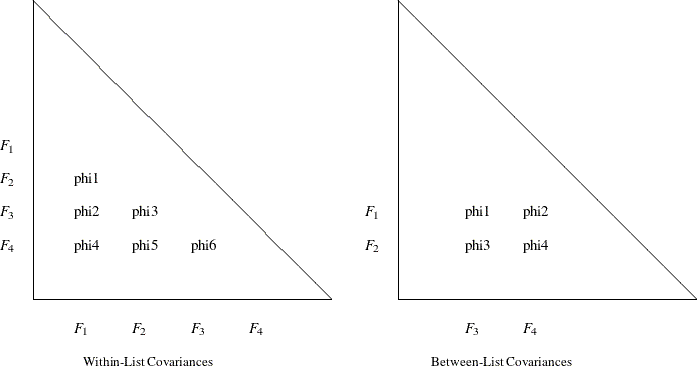
Within-List Covariances
The left panel of Figure 65.9 shows that the same set of four factors is used in both the rows and the columns. This yields six nonredundant covariances
(variances are not included) to specify. In general, for a var-list list that has k variables in the COV statement, you can specify  distinct covariance parameters. The variable order of the var-list list is important. For example, the left panel of Figure 65.9 corresponds to the following COV statement:
cov F1-F4 = phi1-phi6;
This statement is equivalent to the following statement:
cov F2 F1 = phi1,
    F3 F1 = phi2, F3 F2 = phi3,
    F4 F1 = phi4, F4 F2 = phi5, F4 F3 = phi6;
Another way to assign distinct parameter names that have the same prefix is to use the so-called prefix name. For example, the following COV statement is exactly the same as the preceding statement:
cov F1-F4 = 6*phi__; /* phi with two trailing underscores */
In the COV statement, phi_ _ is a prefix name that has the root phi. The notation 6* means that this prefix name is applied six times, resulting in a generation of the six parameter names phi1, phi2, …, phi6 for the six covariance parameters.
The root of the prefix name should have only a few characters so that the generated parameter name is not longer than 32 characters. To avoid unintentional equality constraints, the prefix names should not conflict with other parameter names.
You can also specify the within-list covariances as unnamed free parameters, as shown in the following statement:
cov F1-F4;
This statement is equivalent to the following statement:
cov F2 F1,
    F3 F1, F3 F2,
    F4 F1, F4 F2, F4 F3;
Between-List Covariances
The right panel of Figure 65.9 illustrates the application of the between-list covariance specification. The set of row variables is different from the
set of column variables. You intend to specify the cross covariances of the two sets of variables. There are four of these
covariances in the figure. In general, for  and
and  variable names in the two variable lists (separated by an asterisk) in a COV statement, there are
  distinct covariances to specify. Again, variable order is very important. For example, the right panel of Figure 65.9 corresponds to the following between-list covariance specification:
cov F1 F2 * F3 F4 = phi1-phi4;
This is equivalent to the following statement:
cov  F1 F3 = phi1, F1 F4 = phi2,
     F2 F3 = phi3, F2 F4 = phi4;
You can also use the prefix name specification for the same specification, as shown in the following statement:
cov F1 F2 * F3 F4 = 4*phi__ ; /* phi with two trailing underscores */
Mixed Parameter Lists
You can specify different types of parameters for the list of covariances. For example, you use a list of parameters that have mixed types in the following statement:
cov F1-F4 = phi1(0.1) 0.2 phi3 phi4(0.4) (0.5) phi6;
This statement is equivalent to the following statement:
cov F2 F1 = phi1(0.1) ,
    F3 F1 = 0.2       , F3 F2 = phi3,
    F4 F1 = phi4(0.4) , F4 F2 = (0.5), F4 F3 = phi6;
Notice that an initial value that follows a parameter name is associated with the free parameter. Therefore, in the original
mixed list specification, 0.1 is interpreted as the initial value of the parameter phi1, but not as the initial estimate of the covariance between F3 and F1. Similarly, 0.4 is the initial value of the parameter phi4, but not the initial estimate of the covariance between F4 and F2.
However, if you indeed want to specify that phi1 is a free parameter without an initial value and 0.1 is an initial estimate of the covariance between F3 and F1 (while keeping all other things the same), you can use a null initial value specification for the parameter phi1, as shown in the following statement:
cov F1-F4 = phi1() (0.1) phi3 phi4(0.4) (0.5) phi6;
This way, 0.1 becomes the initial estimate of the covariance between F3 and F1. Because a parameter list that has mixed types might be confusing, you can break down the specifications into separate assignments to remove ambiguities. For example, you can use the following equivalent statement:
cov F2 F1 = phi1 ,
    F3 F1 = (0.1)     , F3 F2 = phi3,
    F4 F1 = phi4(0.4) , F4 F2 = (0.5), F4 F3 = phi6;
Shorter and Longer Parameter Lists
If you provide fewer parameters than the number of covariances in the variable lists, all the remaining parameters are treated
as unnamed free parameters. For example, the following statement assigns a fixed value to cov(F1,F3) while treating all the other three covariances as unnamed free parameters:
cov F1 F2 * F3 F4 = 1.0;
This statement is equivalent to the following statement:
cov F1 F3 = 1.0, F1 F4, F2 F3, F2 F4;
If you intend to fill up all values by the last parameter specification in the list, you can use the continuation syntax [...], [..], or [.], as in the following example:
cov F1 F2 * F3 F4 = 1.0 phi [...];
This means that cov(F1,F3) is a fixed value of 1 and all the remaining three covariances are free parameters named phi. The last three covariances are thus constrained to be equal by having the same parameter name.
However, you must be careful not to provide too many parameters. For example, the following statement results in an error:
cov F1 F2 * F3 F4 = 1.0 phi2(2.0) phi3 phi4 phi5 phi6;
The parameters after phi4 are excessive.
Default Covariance Parameters
In exploratory analysis, all factor covariances are fixed at zero for the unrotated or orthogonally rotated solutions. For confirmatory analysis, by default all factor covariances are fixed at zero. You can also use the COV statement to override these default covariance parameters in situations where you want to set parameter constraints or provide initial or fixed values.