The IRT Procedure
-
Overview

- Getting Started
-
Syntax
-
DetailsNotation for the Item Response Theory ModelAssumptionsPROC IRT Contrasted with Other SAS ProceduresResponse ModelsMarginal LikelihoodApproximating the Marginal LikelihoodMaximizing the Marginal LikelihoodFactor Score EstimationModel and Item FitItem and Test informationMissing ValuesOutput Data SetsODS Table NamesODS Graphics
-
Examples
- References
Approximating the Marginal Likelihood
As discussed in the section Marginal Likelihood, integrations that are involved in the marginal likelihood for IRT model cannot be solved analytically and need to be approximated by using numerical integration, mostly Gauss-Hermite quadrature.
Gauss-Hermite (G-H) Quadrature
In general, the Gauss-Hermite (G-H) quadrature can be presented as
![\[ \int _{-\infty }^{\infty } g(x) \, dx=\int _{-\infty }^{\infty } f(x)\phi (x) \, dx \approx \sum \limits _{g=1}^ G f(x_ g)w_ g \]](images/statug_irt0070.png)
where G is the number of quadrature points and  and
and  are the integration points and weights, respectively, which are uniquely determined by the integration domain and the weighting
kernel
are the integration points and weights, respectively, which are uniquely determined by the integration domain and the weighting
kernel  . Traditional G-H quadrature often uses
  as the weighting kernel. In the field of statistics, the density of standard normal distribution is more widely used instead,
because for estimating various statistical models, the Gaussian density is often a factor of the integrand. In the case in
which the Gaussian density is not a factor of the integrand, the integral is transformed into the form by dividing and multiplying
the original integrand by the standard normal density.
as the weighting kernel. In the field of statistics, the density of standard normal distribution is more widely used instead,
because for estimating various statistical models, the Gaussian density is often a factor of the integrand. In the case in
which the Gaussian density is not a factor of the integrand, the integral is transformed into the form by dividing and multiplying
the original integrand by the standard normal density.
Adaptive Gauss-Hermite Quadrature
The G order G-H quadrature is exact if  is a
is a  degree polynomial in x. However, as many researchers (Lesaffre and Spiessens 2001; Rabe-Hesketh, Skrondal, and Pickles 2002) point out, integrands
 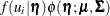 often have sharp peaks and cannot be well approximated by low-degree polynomials in
  . Furthermore, the peak might be far from zero or be located between adjacent quadrature points so that substantial contributions
to the integral are lost.
. Furthermore, the peak might be far from zero or be located between adjacent quadrature points so that substantial contributions
to the integral are lost.
Note that the integrands in the marginal likelihood are a product of the prior density of ,  and the joint probability of responses given ,
  . After normalization with respect to , the integrand, , is just the posterior density of , given the observed responses
  . This posterior density is approximately normal when the number of items is large. Let
  and
and  be the mean and covariance matrix, respectively, of the posterior density. Then the ratio
  can be well approximated by a low-degree polynomial if the number of items is relatively large. This suggests that the integral
should be transformed as
can be well approximated by a low-degree polynomial if the number of items is relatively large. This suggests that the integral
should be transformed as
The integration points and weights that correspond to  are
are
![\[ z_ g = \bSigma _ i^{1/2}x_ g + \bmu _ i \]](images/statug_irt0085.png)
![\[ v_ g = |\bSigma _ i|^{1/2} w_ g \]](images/statug_irt0086.png)
The preceding transformations move and scale the quadrature points to the center of the integrands such that the integrand can be better approximated using many fewer quadrature points.