The IRT Procedure
-
Overview

- Getting Started
-
Syntax
-
DetailsNotation for the Item Response Theory ModelAssumptionsPROC IRT Contrasted with Other SAS ProceduresResponse ModelsMarginal LikelihoodApproximating the Marginal LikelihoodMaximizing the Marginal LikelihoodFactor Score EstimationModel and Item FitItem and Test informationMissing ValuesOutput Data SetsODS Table NamesODS Graphics
-
Examples
- References
Maximizing the Marginal Likelihood
You can obtain parameter estimates by maximizing the marginal likelihood by using either the expectation maximization (EM) algorithm or a Newton-type algorithm. Both algorithms are available in PROC IRT.
The most widely used estimation method for IRT models is the Gauss-Hermite quadrature–based EM algorithm, proposed by Bock and Aitkin (1981). However, this method has several important shortcomings, the most serious of which is the lack of reliable convergence criteria. Without reliable convergence criteria, estimates can be seriously biased because of spurious convergence. In comparison, gradient-based convergence criteria is readily available for Newton-type algorithms. As a result, PROC IRT uses the quasi-Newton algorithm instead of EM as the default optimization method.
Newton-Type Algorithms
Newton-type algorithms maximize the marginal likelihood directly, based on the first and second derivatives. Two of the most widely used estimation algorithms are the Newton-Raphson and Fisher scoring algorithms, which rely on the gradient and Hessian of the log likelihood. However, for latent variable models that contain categorical responses, the Hessian matrix is often expensive to compute. As a result, several quasi-Newton algorithms that require only gradients have been proposed. In the field of IRT, Bock and Lieberman (1970) propose replacing the Hessian with the following information matrix:
![\[ I(\btheta ) = E\left[\frac{\partial \log \tilde{L}(\theta |U)}{\partial \theta }\left(\frac{\partial \log \tilde{L}(\theta |U)}{\partial \theta }\right)^ T\right] = \sum _{h=1}^{2^ J}\left[\frac{\partial \log \tilde{L}_ i}{\partial \theta }\left(\frac{\partial \log \tilde{L}_ i}{\partial \theta }\right)^ T\right] \]](images/statug_irt0087.png)
To calculate the preceding expectation, you need to sum over not just the observed but all  possible response patterns; this becomes computationally very expensive when the number of items is large. Fortunately, other
quasi-Newton algorithms that do not have these computational difficulties have been proposed. The Broyden-Fletcher-Goldfarb-Shanno
(BFGS) method is one of the most popular quasi-Newton algorithms that approximate the Hessian matrix with gradient.
possible response patterns; this becomes computationally very expensive when the number of items is large. Fortunately, other
quasi-Newton algorithms that do not have these computational difficulties have been proposed. The Broyden-Fletcher-Goldfarb-Shanno
(BFGS) method is one of the most popular quasi-Newton algorithms that approximate the Hessian matrix with gradient.
For the objective function,  , the first derivatives with respect to
  are
are
![\begin{equation*} \frac{\partial \log \tilde{L}(\btheta |\mb{U})}{\partial \theta _ j} = \sum _{i=1}^ N \left[(\tilde{L}_ i)^{-1}\frac{\partial \tilde{L}_ i}{\partial \theta _ j}\right] =\sum _{i=1}^ N\left[(\tilde{L}_ i)^{-1}\sum _{g=1}^{G^ d}\left[\frac{\partial f_ i(\mb{x}_ g)}{\partial \theta _ j}w^{*}_ g\right]\right] \end{equation*}](images/statug_irt0091.png)
where
![\begin{equation*} \tilde{L}_ i = \sum _{g=1}^{G^ d}\left[\prod _{j=1}^ J \prod _{k=1}^ K(P_{ijk}(\mb{x}_ g))^{v_{ijk}}\frac{\phi (\mb{x}_ g;\bmu ,\bSigma )}{d(\mb{x}_ g;0,I)}\right]w_ g = \sum _{g=1}^{G^ d} f_ i(x_ g)w_ g \end{equation*}](images/statug_irt0092.png)
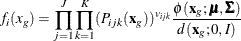
and
![\begin{equation*} \frac{\partial f_ i(\mb{x}_ g)}{\partial \theta _{Ij}} = \frac{\partial [(P_{ijk}(\mb{x}_ g))]}{\partial \theta _ j} \frac{f_ i(\mb{x}_ g)}{(P_{ijk}(\mb{x}_ g))} \end{equation*}](images/statug_irt0094.png)
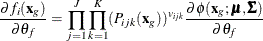
where, in the preceding two equations,  indicate parameters that are associated with item j and
  represents parameters that are related to latent factors.
Expectation-Maximization (EM) Algorithm
The expectation-maximization (EM) algorithm starts from the complete data log likelihood that can be expressed as follows:
![\[ \begin{array}{lll} \log L(\btheta |\mb{U},\bm {\eta }) & =& \sum \limits _{i=1}^ N\left[\sum \limits _{j=1}^ J\sum \limits _{k=1}^ K v_{ijk}\log P_{ijk} + \log \phi (\bm {\eta }_ i;\bmu ,\bSigma ) \right]\\ & =& \sum \limits _{j=1}^ J\sum \limits _{i=1}^ N\left[\sum \limits _{k=1}^ K v_{ijk}\log P_{ijk}\right] + \sum \limits _{i=1}^ N \log \phi (\bm {\eta }_ i;\bmu ,\bSigma ) \end{array} \]](images/statug_irt0098.png)
The expectation (E) step calculates the expectation of the complete data log likelihood with respect to the conditional distribution
of  ,
,  as follows:
![\[ Q(\btheta |\btheta ^{(t)}) = \sum \limits _{j=1}^ J\sum \limits _{i=1}^ N\left[\sum \limits _{k=1}^ Kv_{ijk}E\left[\log P_{ijk}|\mb{u}_ i,\btheta ^{(t)}\right]\right] + \sum \limits _{i=1}^ N E\left[\log \phi (\bm {\eta }_ i;\bmu ,\bSigma )|\mb{u}_ i,\btheta ^{(t)}\right] \]](images/statug_irt0100.png)
The conditional distribution  is
is
![\[ f(\bm {\eta }|\mb{u}_ i,\btheta ^{(t)}) = \frac{f(\mb{u}_ i|\bm {\eta },\btheta ^{(t)})\phi (\bm {\eta };\bmu ^{(t)},\bSigma ^{(t)})}{\int f(\mb{u}_ i|\bm {\eta },\btheta ^{(t)})\phi (\bm {\eta };\bmu ^{(t)},\bSigma ^{(t)})\, d\bm {\eta } } = \frac{f(\mb{u}_ i|\bm {\eta },\btheta ^{(t)})\phi (\bm {\eta }; \bmu ^{(t)},\bSigma ^{(t)})}{f(\mb{u}_ i)} \]](images/statug_irt0102.png)
These conditional expectations that are involved in the Q function can be expressed as follows:
![\begin{equation*} E[\log P_{ijk}|\mb{u}_ i,\btheta ^{(t)}] = \int \log P_{ijk}f(\bm {\eta }|\mb{u}_ i,\btheta ^{(t)})\, d\bm {\eta } \end{equation*}](images/statug_irt0103.png)
![\begin{equation*} E[\log \phi (\bm {\eta };\bmu ,\bSigma )|\mb{u}_ i,\btheta ^{(t)}] = \int \log \phi (\bm {\eta };\bmu ,\bSigma )f(\bm {\eta }|\mb{u}_ i,\btheta ^{(t)})\, d\bm {\eta } \end{equation*}](images/statug_irt0104.png)
Then
![\[ Q(\btheta |\btheta ^{(t)}) = \sum \limits _{j=1}^ J\int \left[\log P_{ijk}r_{jk}(\btheta ^{(t)})\right]\phi (\bm {\eta };\bmu ^{(t)},\bSigma ^{(t)}) \, d\bm {\eta } + \int \log \phi (\bm {\eta }|\btheta ) N(\btheta ^{(t)}) \phi (\bm {\eta };\bmu ^{(t)},\bSigma ^{(t)})\, d\bm {\eta } \]](images/statug_irt0105.png)
where
![\[ r_{jk}(\btheta ^{(t)})=\sum \limits _{i=1}^ N \sum \limits _{k=1}^ K v_{ijk}\frac{f(\mb{u}_ i|\eta ,\btheta ^{(t)})}{f(\mb{u}_ i)} \]](images/statug_irt0106.png)
and
![\[ N(\btheta ^{(t)})=\sum \limits _{i=1}^ N \frac{f(\mb{u}_ i|\bm {\eta },\btheta ^{(t)})}{f(\mb{u}_ i)} \]](images/statug_irt0107.png)
Integrations in the preceding equations can be approximated as follows by using G-H quadrature:
![\[ \tilde{Q}(\btheta |\btheta ^{(t)}) = \sum _{g=1}^{G}\left[\log P_{ijk}(\mb{x}_ g)r_{jk}(\mb{x}_ g, \btheta ^{(t)})+\log \phi (\mb{x}_ g|\btheta )N(\mb{x}_ g,\btheta ^{(t)})\right] \frac{\phi (\mb{x}_ g;\bmu ^{(t)}, \bSigma ^{(t)})}{d(\mb{x}_ g;0,I)} w_ g \]](images/statug_irt0108.png)
In the maximization (M) step of the EM algorithm, parameters are updated by maximizing  . To summarize, the EM algorithm consists of the following two steps:
-
E step: Approximate
 by using numerical integration.
-
M step: Update parameter estimates by maximizing
 with the one-step Newton-Raphson algorithm.