The HPSPLIT Procedure

This example illustrates how you can use the HPSPLIT procedure to build and assess a classification tree for a binary outcome. Overfitting is avoided by cost-complexity pruning, and the selection of the pruning parameter is based on cross validation.

The training data in this example come from the Lichen Air Quality Surveys (Geiser and Neitlich 2007), which were conducted in western Oregon and Washington between 1994 and 2001. Both the training data and the test data in this example were provided by Richard Cutler, Department of Mathematics and Statistics, Utah State University.

The following statements create a data set named LAQ that provides 30 measurements of environmental conditions such as temperature, elevation, and moisture at 840 sites. These variables are treated as predictors for the response variable LobaOreg, which is coded as 1 if the lichen species Lobaria oregana was present at the site and 0 otherwise.

data LAQ;
   length ReserveStatus $ 9;
   input LobaOreg Aconif DegreeDays TransAspect Slope Elevation
         PctBroadLeafCov PctConifCov PctVegCov TreeBiomass EvapoTransAve
         EvapoTransDiff MoistIndexAve MoistIndexDiff PrecipAve PrecipDiff
         RelHumidAve RelHumidDiff PotGlobRadAve PotGlobRadDiff AveTempAve
         AveTempDiff DayTempAve DayTempDiff MinMinTemp MaxMaxTemp
         AmbVapPressAve AmbVapPressDiff SatVapPressAve SatVapPressDiff
         ReserveStatus $;
   datalines;
     0 44.897  24737 0.5174      1   1567     12     80     92     89 23.333
    36 182.65  -2037 89.623 -93.49 57.476 -11.02  19438  15935 6.5028 10.342
7.9045 10.925  -5.97  25.36 637.68    350 1166.1 836.84 Matrix

   ... more lines ...   

     0 248.55  20628 0.6954     25   1106      0    100     98    200 18.944
28.748 1495.6  -2840 207.48 -196.1  68.15 -8.207  18032  14569 5.6545 8.4487
6.6142 8.8087 -4.123 19.769 689.34 334.93 1035.1 616.72 Reserve
;

proc print data=LAQ(obs=5);
   var LobaOreg MinMinTemp Aconif PrecipAve Elevation ReserveStatus;
run;

Output 61.1.1 lists the first five observations for six of the variables in LAQ.

The following statements invoke the HPSPLIT procedure to create a classification tree for LobaOreg:

ods graphics on;

proc hpsplit data=LAQ seed=123;
   class LobaOreg ReserveStatus;
   model LobaOreg (event='1') =
      Aconif DegreeDays TransAspect Slope Elevation PctBroadLeafCov
      PctConifCov PctVegCov TreeBiomass EvapoTransAve EvapoTransDiff
      MoistIndexAve MoistIndexDiff PrecipAve PrecipDiff RelHumidAve
      RelHumidDiff PotGlobRadAve PotGlobRadDiff AveTempAve AveTempDiff
      DayTempAve DayTempDiff MinMinTemp MaxMaxTemp AmbVapPressAve
      AmbVapPressDiff SatVapPressAve SatVapPressDiff ReserveStatus;
   grow entropy;
   prune costcomplexity;
run;

In the case of binary outcomes, the EVENT= option is used to explicitly control the level of the response variable that represents the event of interest for computing the area under the curve (AUC), sensitivity, specificity, and values of the receiver operating characteristic (ROC) curves.

Note: These fit statistics do not apply to categorical response variables that have more than two levels, so the EVENT= option does not apply in that situation. Likewise, this option does not apply to continuous response variables.

The GROW statement specifies the entropy criterion for splitting the observations during the process of recursive partitioning that results in a large initial tree. The PRUNE statement requests cost-complexity pruning to select a smaller subtree that avoids overfitting the data.

The plot in Output 61.1.2 displays estimates of the average square error (ASE) for a series of progressively smaller subtrees of the large tree that are indexed by a cost-complexity parameter that is also referred to as a pruning or tuning parameter. The plot provides a tool for selecting the parameter that results in the smallest estimated ASE.

Output 61.1.2: ASE as a Function of Cost-Complexity Parameter

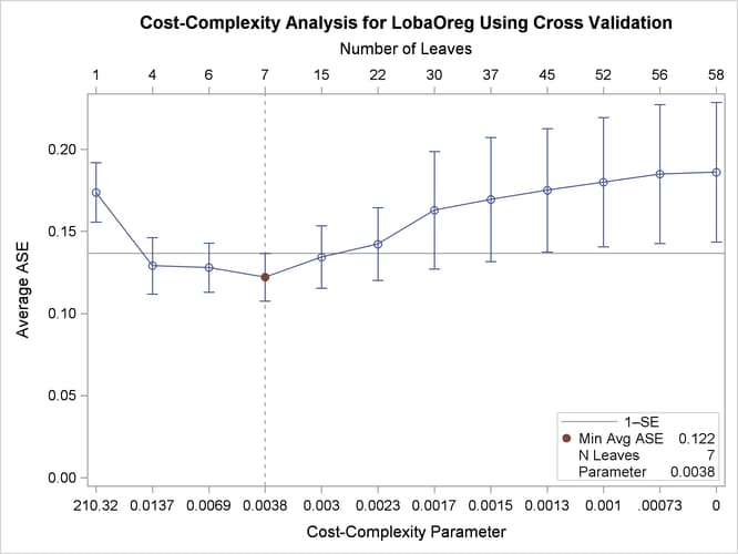
The ASEs are estimated by 10-fold cross validation; for computational details, see the section Cost-Complexity Pruning. The subtree size (number of leaves) that corresponds to each parameter is indicated on the upper horizontal axis. The parameter value 0 corresponds to the fully grown tree, which has 58 leaves.

By default, PROC HPSPLIT selects the parameter that minimizes the ASE, as indicated by the vertical reference line and the dot in Output 61.1.2. Here the minimum ASE occurs at a parameter value of 0.0038, which corresponds to a subtree with seven leaves. However, the ASEs for two smaller subtrees, one with four leaves and one with six leaves, are indistinguishable from the minimum ASE. This is evident from a comparison of the standard errors for the ASEs, which are represented by the error bars.

In general, the plot in Output 61.1.2 often shows parameter choices that correspond to smaller subtrees for which the ASEs are nearly the same as the minimum ASE. A common approach for choosing the parameter is the 1-SE rule of Breiman et al. (1984), which selects the smallest subtree for which the ASE is less than the minimum ASE plus one standard error. In this case, the 1-SE rule selects a subtree that has only four leaves, but this is such a small subtree that the subtree with six leaves and a parameter value of 0.0069 seems preferable.

Note: The estimated ASEs and their standard errors depend on the random allocation of the observations to the 10 folds. You obtain different estimates if you specify a different SEED= value. Likewise, the estimates differ if you request a different number of folds by using the CVMETHOD= option.

The following statements rerun the analysis and request a tree with six leaves:

proc hpsplit data=LAQ cvmodelfit seed=123;
   class LobaOreg ReserveStatus;
   model LobaOreg (event='1') =
      Aconif DegreeDays TransAspect Slope Elevation PctBroadLeafCov
      PctConifCov PctVegCov TreeBiomass EvapoTransAve EvapoTransDiff
      MoistIndexAve MoistIndexDiff PrecipAve PrecipDiff RelHumidAve
      RelHumidDiff PotGlobRadAve PotGlobRadDiff AveTempAve AveTempDiff
      DayTempAve DayTempDiff MinMinTemp MaxMaxTemp AmbVapPressAve
      AmbVapPressDiff SatVapPressAve SatVapPressDiff ReserveStatus;
   grow entropy;
   prune costcomplexity(leaves=6);
   code file='trescore.sas';
run;

The tree diagram in Output 61.1.3 provides an overview of the entire tree.

Output 61.1.3: Overview of Fitted Tree

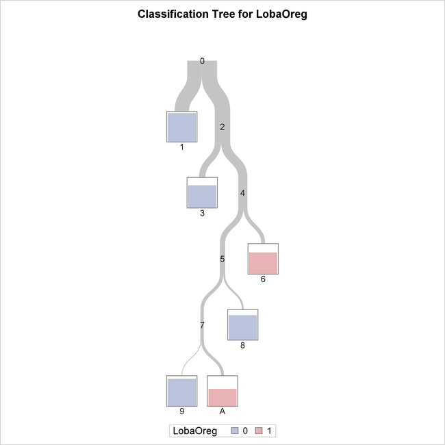
The color of the bar in each leaf node indicates the most frequent level of LobaOreg and represents the classification level assigned to all observations in that node. The height of the bar indicates the proportion of observations (sites) in the node that have the most frequent level.

The diagram in Output 61.1.4 provides more detail about the nodes and splits in the first four levels of the tree. It reveals a model that is highly interpretable.

Output 61.1.4: First Four Levels of Fitted Tree

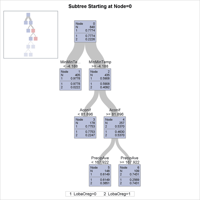
The first split is based on the variable MinMinTemp, which is the minimum of the 12 monthly minimum temperatures at each site. There are 405 sites whose values of MinMinTemp are less than –4.188 (node 1), and the species Lobaria oregana is present at only around 2% of them. Apparently this species does not grow well when the temperature can get very low.

The 435 sites for which MinMinTemp –4.188 (node 2) are further subdivided based on the variable Aconif, which is the average age of the dominant conifer at the site. Lobaria oregana is present at 53.7% of the 257 sites for which MinMinTemp –4.188 and Aconif 81.896 years. The cutoff of 81.896 years is notable because coniferous forests in the Pacific Northwest begin to exhibit old-forest characteristics at approximately 80 years of age (Old-Growth Definition Task Group 1986), and Lobaria oregana is a lichen species that is associated with old forests.

The 257 sites for which Aconif 81.896 are further subdivided on the basis of PrecipAve (average monthly precipitation) with a cutoff value 167.922 mm. Lobaria oregana was present at 74.31% of the 109 sites for which MinMinTemp –4.188, Aconif 81.896 years, and PrecipAve 167.922 mm. Contrast this occupancy percentage with the 2.22% for the sites for which MinMinTemp –4.188.

In summary, based on the first three splits, Lobaria oregana is most likely to be found at sites for which MinMinTemp –4.188, Aconif 81.896, and PrecipAve 167.922.

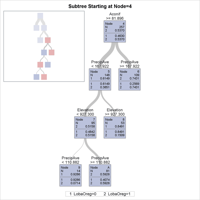
The following statements use the PLOTS=ZOOMEDTREE option to request a detailed diagram of the subtree that begins at node 4:

proc hpsplit data=LAQ cvmodelfit seed=123
   plots=zoomedtree(nodes=('4') depth=4);
   class LobaOreg ReserveStatus;
   model LobaOreg (event='1') =
      Aconif DegreeDays TransAspect Slope Elevation PctBroadLeafCov
      PctConifCov PctVegCov TreeBiomass EvapoTransAve EvapoTransDiff
      MoistIndexAve MoistIndexDiff PrecipAve PrecipDiff RelHumidAve
      RelHumidDiff PotGlobRadAve PotGlobRadDiff AveTempAve AveTempDiff
      DayTempAve DayTempDiff MinMinTemp MaxMaxTemp AmbVapPressAve
      AmbVapPressDiff SatVapPressAve SatVapPressDiff ReserveStatus;
   grow entropy;
   prune costcomplexity(leaves=6);
   code file='trescore.sas';
run;

This subtree, shown in Output 61.1.5, provides details for the portion of the entire tree that is not shown in Output 61.1.4.

Output 61.1.5: Bottom Four Levels of Fitted Tree

Note: You can use the NODES= option to request a table that describes the path from each leaf in the fitted tree back to the root node.

The next three displays evaluate the accuracy of the selected classification tree. Output 61.1.6 provides two confusion matrices.

The model-based confusion matrix is sometimes referred to as a resubstitution confusion matrix, because it results from applying the fitted model to the training data. The cross validation confusion matrix is produced when you specify the CVMODELFIT option. It is based on a 10-fold cross validation that is done independently of the 10-fold cross validation that is used to estimate ASEs for pruning parameters.

The table in Output 61.1.7 provides fit statistics for the selected classification tree.

Two sets of fit statistics are provided. The first is based on the fitted model, and the second (requested by the CVMODELFIT option) is based on 10-fold cross validation.

The model-based misclassification rate is low (14.2%), but the corresponding sensitivity, which measures the prediction accuracy at sites where the species is present, is only 69%. Good overall prediction accuracy but poor prediction of a particular level can occur when the data are not well balanced (in this case there are three times as many sites where the species is absent as there are sites where the species is present).

The cross validation misclassification rate is higher (18.1%) than the model-based rate, and the cross validation sensitivity is 64%, which is lower than the model-based sensitivity. Model-based error rates tend to be optimistic.

Output 61.1.8 displays an ROC curve, which is produced only for binary outcomes.

Output 61.1.8: ROC Curve for Classification of LAQ

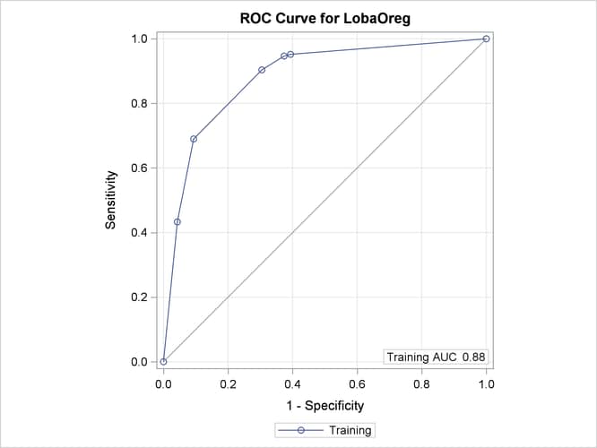
The AUC statistic and the values of the ROC curve are computed from the training data. When you specify a validation data set by using the PARTITION statement, the plot displays an additional ROC curve and AUC statistic, whose values are computed from the validation data.

Note: In this example, the computations of the sensitivity, specificity, AUC, and values of the ROC curve depend on defining LobaOreg=1 as the event of interest by using the EVENT= option in the MODEL statement.

Another way to assess the predictive accuracy of the fitted tree is to apply it to an independent test data set. In 2003, data on the presence of Lobaria oregana were collected at 300 sites as part of the Survey and Manage Program within the Northwest Forest Plan, the conservation plan for the northern spotted owl (Molina et al. 2003). These sites were in approximately the same area where the earlier Lichen Air Quality Surveys were conducted, with similar (but not identical) sampling protocols. The 2003 surveys are sometimes called the Pilot Random Grid surveys (Edwards et al. 2005). Lobaria oregana was detected at 26.7% (80) of the sites, an occupancy rate comparable to that of the Lichen Air Quality Surveys (187 / 840 = 22.3%).

The following DATA step reads the data from the Pilot Random Grid surveys:

data PRG;
   length ReserveStatus $ 9;
   input LobaOreg ACONIF DegreeDays TransAspect Slope Elevation
         PctBroadLeafCov PctConifCov PctVegCov TreeBiomass EvapoTransAve
         EvapoTransDiff MoistIndexAve MoistIndexDiff PrecipAve PrecipDiff
         RelHumidAve RelHumidDiff PotGlobRadAve PotGlobRadDiff AveTempAve
         AveTempDiff DayTempAve DayTempDiff MinMinTemp MaxMaxTemp
         AmbVapPressAve AmbVapPressDiff SatVapPressAve SatVapPressDiff
         ReserveStatus $;
   datalines;
     0 97.834  30901 0.9045     25   1086 9.0581 71.347 89.852    150 28.917
  35.5    142  -2105 1024.8  -1019 614.75 -116.2  21837  13799 844.33    876
969.58 931.17   -218   2521 758.25  333.5 1284.8 788.33 Reserve

   ... more lines ...   

     0     10  18109 0.6628     26   1344     25     44     69     85  16.75
  27.5 1753.5  -3008 2266.3  -2168 690.42 -77.83  17610  15299 462.33    836
554.17 869.67   -496   1849 650.17    320 961.67    572 Reserve
;

The CODE statement in the preceding PROC HPSPLIT step requests a file named trescore.sas that contains SAS DATA step code for the rules that define the fitted tree model. You can use this code to classify the observations in the PRG data set as follows:

data lichenpred(keep=Actual Predicted);
   set PRG end=eof;
   %include "trescore.sas";
   Actual    = LobaOreg;
   Predicted = (P_LobaOreg1 >= 0.5);
run;

The variables P_LobaOreg1 and P_LobaOreg0 contain the predicted probabilities that Lobaria oregana is present or absent, respectively. The value of the expression (P_LobaOreg1 >= 0.5) is 1 when P_LobaOreg1 P_LobaOreg0.

The following statements use these probabilities to produce a confusion matrix:

title "Confusion Matrix Based on Cutoff Value of 0.5";
proc freq data=lichenpred;
   tables Actual*Predicted / norow nocol nopct;
run;

The matrix is shown in Output 61.1.9.

The misclassification rate is (40 + 29) / 300 = 0.23, which is higher than the rates in Output 61.1.7. The sensitivity is 50%, which is less than the cross validation sensitivity in Output 61.1.7. The specificity is 86.8%.

When the sensitivity is much smaller than the specificity (which is common for highly unbalanced data), you can change the probability cutoff to a smaller value, increasing the sensitivity at the expense of the specificity and the overall accuracy. The following statements produce the confusion matrix for a cutoff value of 0.1:

data lichenpred(keep=Actual Predicted);
   set PRG end=eof;
   %include "trescore.sas";
   Actual    = LobaOreg;
   Predicted = (P_LobaOreg1 >= 0.1);
run;

title "Confusion Matrix Based on Cutoff Value of 0.1";
proc freq data=lichenpred;
   tables Actual*Predicted / norow nocol nopct;
run;

The matrix is shown in Output 61.1.10.

Based on the cutoff value of 0.1, the sensitivity is 56.3% and the specificity is 72.7%.