The HPSPLIT Procedure

Pruning
The HPSPLIT procedure creates a classification or regression tree by first growing a tree as described in the section Splitting Criteria. This usually results in a large tree that provides a good fit to the training data. The problem with this tree is its potential for overfitting the data: the tree can be tailored too specifically to the training data and not generalize well to new data. The solution is to find a smaller subtree that results in a low error rate on holdout or validation data.
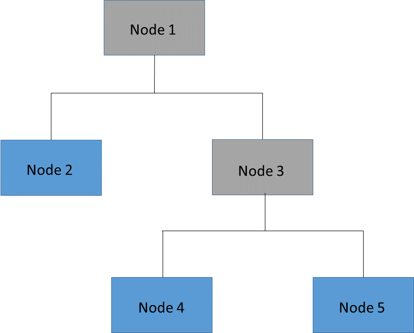
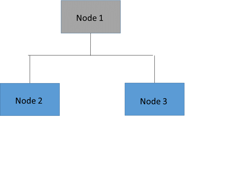
It is often prohibitively expensive to evaluate the error on all possible subtrees of the full tree. A more practical strategy is to focus on a sequence of nested trees obtained by successively pruning leaves from the tree. Figure 61.14 shows an example of pruning in which the leaves (or terminal nodes) of Node 3 (Nodes 4 and 5) are removed to create a nested subtree of the full tree. In the nested subtree, Node 3 is now a leaf that contains all the observations that were previously in Nodes 4 and 5. This process is repeated until only the root node remains.
Figure 61.14: Tree and Pruned Subtree
|
Full Tree |
Nested Subtree (Node 3 Pruned) |
|
|
|
Many different methods have been proposed for pruning in this manner. These methods address both how to select which nodes to prune to create the sequence of subtrees and how then to select the optimal subtree from this sequence as the final tree. You can use the PRUNE statement in PROC HPSPLIT to specify which pruning method to apply and related options. Several well-known pruning methods, described in this section, are available, and you can override the final selected tree based on your preferences or domain knowledge.
Cost-Complexity Pruning
Cost-complexity pruning is a widely used pruning method that was originally proposed by Breiman et al. (1984). You can request cost-complexity pruning for either a categorical or continuous response variable by specifying
prune costcomplexity;
This algorithm is based on making a trade-off between the complexity (size) of a tree and the error rate to help prevent overfitting. Thus large trees with a low error rate are penalized in favor of smaller trees. The cost complexity of a tree T is defined as
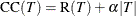
where R(T) represents its error rate, |T| represents the number of leaves on T, and the complexity parameter  represents the cost of each leaf. For a categorical response variable, the misclassification rate is used for the error rate,
R(T); for a continuous response variable, the residual sum of squares (RSS), also called the sum of square errors (SSE), is used
for the error rate. Note that only the training data are used to evaluate cost complexity.
represents the cost of each leaf. For a categorical response variable, the misclassification rate is used for the error rate,
R(T); for a continuous response variable, the residual sum of squares (RSS), also called the sum of square errors (SSE), is used
for the error rate. Note that only the training data are used to evaluate cost complexity.
Breiman et al. (1984) show that for each value of , there is a subtree of T that minimizes cost complexity. When  , this is the full tree,
  . As increases, the corresponding subtree becomes progressively smaller, and the subtrees are in fact nested. Then, at some value
of , the root node has the minimal cost complexity for any greater than or equal to that value. Because there are a finite number of possible subtrees, each subtree corresponds to
an interval of values of ; that is,
. As increases, the corresponding subtree becomes progressively smaller, and the subtrees are in fact nested. Then, at some value
of , the root node has the minimal cost complexity for any greater than or equal to that value. Because there are a finite number of possible subtrees, each subtree corresponds to
an interval of values of ; that is,
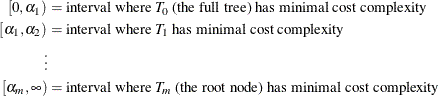
PROC HPSPLIT uses weakest-link pruning, as described by Breiman et al. (1984), to create the sequence of  values and the corresponding sequence of nested subtrees,
  .
.
Finding the optimal subtree from this sequence is then a question of determining the optimal value of the complexity parameter
. This is performed either by using the validation partition, when you use the PARTITION statement to reserve a validation
holdout sample, or by using cross validation. In the first case, the subtree in the pruning sequence that has the lowest validation
error rate is selected as the final tree. When there is no validation partition, k-fold cross validation can be applied to cost-complexity pruning to select a subtree that generalizes well and does not overfit
the training data (Breiman et al. 1984; Zhang and Singer 2010). The algorithm proceeds as follows after creating the sequence of subtrees and values by using the entire set of training data as described earlier:
-
Randomly divide the training observations into k approximately equal-sized parts, or folds.
-
Define a sequence of
 values as the geometric mean of the endpoints of the
  intervals (that is,
  ) to represent the intervals.
-
For each of the k folds, hold out the current fold for validation and use the remaining
 folds for the training data in the following steps:
-
Grow a tree as done using the full training data set with the same splitting criterion.
-
Using the
 values that are calculated in step 2, create a sequence of subtrees for each
  as described in the pruning steps given earlier, but now using as a fixed value for and minimizing the cost complexity, CC(T), to select a subtree at each pruning step.
-
For each
, set  to be the subtree that has the minimum cost complexity from the sequence for the jth fold.
-
Calculate the error
 for each by using the current (jth) fold (the one omitted from the training).
-
-
Now the error rate can be averaged across folds,
 , and the that has the smallest
  is selected. The tree
  from pruning the complete training data that corresponds to the selected is the final selected subtree.
The HPSPLIT procedure provides two plots that you can use to tune and evaluate the pruning process: the cost-complexity analysis plot and the cost-complexity pruning plot.
When performing cost-complexity pruning with cross validation (that is, no PARTITION statement is specified), you should examine
the cost-complexity analysis plot that is created by default. This plot displays as a function of the complexity parameters , and it uses a vertical reference line to indicate the that minimizes . You can use this plot to examine alternative choices for . For example, you might prefer to select a smaller tree that has only a slightly higher error rate. The plot also gives you
the information that you need to implement the 1-SE rule developed by Breiman et al. (1984).
You can use the LEAVES= option in the PRUNE statement to select a tree that has a specified number of leaves. This is illustrated in Example 61.2: Cost-Complexity Pruning with Cross Validation.
When you specify validation data by using the PARTITION statement, the cost-complexity pruning plot displays the error rate R(T) as a function of the number of leaves |T| for both the training and validation data. This plot indicates the final selected tree, the tree with the minimum R(T) for the validation data, by using a vertical reference line. Like the cost-complexity analysis plot that is produced when you perform cross validation, this plot can help you identify a smaller tree that has only a slightly higher validation error rate. You could then use the LEAVES= option in a subsequent run of PROC HPSPLIT to obtain the final selected tree that has the number of leaves that you specify. See Output 61.4.7 in Example 61.4: Creating a Binary Classification Tree with Validation Data for an example of this plot.
C4.5 Pruning
Quinlan (1987) first introduced pessimistic pruning as a pruning method for classification trees in which the estimate of the true error rate is increased by using a statistical correction in order to prevent overfitting. C4.5 pruning (Quinlan 1993) then evolved from pessimistic pruning to employ an even more pessimistic (that is, higher) estimate of the true error rate. An advantage of methods like pessimistic and C4.5 pruning is that they enable you to use all the data for training instead of requiring a holdout sample. In C4.5 pruning, the upper confidence limit of the true error rate based on the binomial distribution is used to estimate the error rate. The C4.5 algorithm variant that PROC HPSPLIT implements uses the beta distribution in place of the binomial distribution for estimating the upper confidence limit. This pruning method is available only for categorical response variables and is implemented when you specify
prune C45;
The C4.5 pruning method follows these steps:
-
Grow a tree from the training data set, and call this full, unpruned tree
.
-
Solve the following equation for
 , the adjusted prediction error rate for leaf l, for each leaf in the tree:
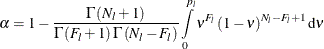
Here the confidence level
is specified in the CONFIDENCE= option,  is the number of failures (misclassified observations) at leaf l,
  is the number of observations at leaf l, and the function
  is defined as
-
Given these values of
, use the formula for the prediction error E of a tree T to calculate  for the full tree before pruning:

-
Consider all nodes that have only leaves as children for pruning in tree
.
-
Calculate the prediction error for each possible subtree that is created by replacing a node with a leaf by using the equations from steps 2 and 3, and prune the node that creates the subtree that has the largest decrease (or smallest increase) in prediction error from tree
. Let this be the next subtree in the sequence,  .
.
-
Repeat steps 2–5 with subtree
from step 5 as the new "full" tree to use for creating the next subtree in the sequence,  . Continue until only the root node remains, represented by
  .
.
The change in error is calculated between each pair of consecutive subtrees,  . For the first change
  that is greater than 0, for
  , subtree
  is selected as the final subtree. Note that for subtree selection, the change in error is calculated on the validation partition when it exists; otherwise the training data are used.
Reduced-Error Pruning
Quinlan’s reduced-error pruning (1987) performs pruning and subtree selection based on minimizing the error rate in the validation partition at each pruning step and then in the overall subtree sequence. This is usually based on the misclassification rate for a categorical response variable, but the average square error (ASE) can also be used. For a continuous response, the error is measured by the ASE. To implement reduced-error pruning, you can use the following PRUNE statement:
prune reducederror;
This pruning algorithm is implemented as follows, starting with the full tree, :
-
Consider all nodes that have only leaves as children for pruning in tree
.
-
For each subtree that is created by replacing a node from step 1 with a leaf, calculate the error rate by using the validation data when available (otherwise use the training data).
-
Replace the node that has the smallest error rate with a leaf, and let
be the subtree.
-
Repeat steps 1–3 with subtree
from step 3 as the new "full" tree to use for creating the next subtree in the sequence, . Continue until only the root node remains, represented by .
This algorithm creates a sequence of subtrees from the largest tree, , to the root node, . The subtree that has the smallest validation error is then selected as the final subtree. Note that using this method without
validation data results in the largest tree being selected. Also note that pruning could be stopped as soon as the error starts
to increase in the validation data as originally described by Quinlan; continuing to prune to create a subtree sequence back
to the root node enables you to select a smaller tree that still has an acceptable error rate, as discussed in the next section.
User Specification of Subtree
There might be situations in which you want to select a different tree from the one selected by default but using cost-complexity or reduced-error pruning to create the sequence of subtrees. For example, maybe there is a subtree that has a slightly larger error but is smaller, and thus simpler, than the subtree with the minimum ASE that was selected using reduced-error pruning. In that case, you can override the selected subtree and instead select the subtree with n leaves that was created using cost-complexity or reduced-error pruning, where n is specified in the LEAVES= option in the PRUNE statement. You can implement the 1-SE rule for cost-complexity pruning described by Breiman et al. (1984) by using this option, as shown in Example 61.2: Cost-Complexity Pruning with Cross Validation. Alternatively, you might want to select the largest tree that is created. In this case, you have two options: you can specify LEAVES=ALL in the PRUNE statement to still see the statistics for the sequence of subtrees created according to the specified pruning error measure, but the tree with no pruning performed is selected as the final subtree; or you can specify
prune off;
to select the largest tree with no pruning performed, meaning that statistics are not calculated and plots are not created on a sequence of subtrees.