The HPSPLIT Procedure

Splitting Criteria
The goal of recursive partitioning, as described in the section Building a Decision Tree, is to subdivide the predictor space in such a way that the response values for the observations in the terminal nodes are
as similar as possible. The HPSPLIT procedure provides two types of criteria for splitting a parent node  : criteria that maximize a decrease in node impurity, as defined by an impurity function, and criteria that are defined by
a statistical test. You select the criterion by specifying an option in the GROW
statement.
: criteria that maximize a decrease in node impurity, as defined by an impurity function, and criteria that are defined by
a statistical test. You select the criterion by specifying an option in the GROW
statement.
Criteria Based on Impurity
The entropy, Gini index, and RSS criteria decrease impurity. The impurity of a parent node is defined as  , a nonnegative number that is equal to zero for a pure node—in other words, a node for which all the observations have the
same value of the response variable. Parent nodes for which the observations have very different values of the response variable
have a large impurity.
, a nonnegative number that is equal to zero for a pure node—in other words, a node for which all the observations have the
same value of the response variable. Parent nodes for which the observations have very different values of the response variable
have a large impurity.
The HPSPLIT procedure selects the best splitting variable and the best cutoff value to produce the highest reduction in impurity,
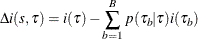
where  denotes the bth child node, p(|) is the proportion of observations in that are assigned to , and B is the number of branches after splitting .
The impurity reduction criteria available for classification trees are based on different impurity functions i() as follows:
-
Entropy criterion (default)
The entropy impurity of node
is defined as
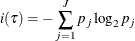
where
 is the proportion of observations that have the jth response value.
-
Gini index criterion
The Gini index criterion defines i(
) as the Gini index that corresponds to the ASE of a class response and is given by

For more information, see Hastie, Tibshirani, and Friedman (2009).
The impurity reduction criterion available for regression trees is as follows:
-
RSS criterion (default)
The RSS criterion, also referred to as the ANOVA criterion, defines i(
) as the residual sum of squares
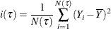
where
 is the number of observations in ,
  is the response value of observation i, and
  is the average response of the observations in .
Criteria Based on Statistical Test
The chi-square, F test, CHAID, and FastCHAID criteria are defined by statistical tests. These criteria calculate the worth of a split by testing
for a significant difference in the response variable across the branches defined by a split. The worth is defined as  , where p is the p-value of the test. You can adjust the p-values for these criteria by specifying the BONFERRONI option in the GROW
statement.
, where p is the p-value of the test. You can adjust the p-values for these criteria by specifying the BONFERRONI option in the GROW
statement.
The criteria based on statistical tests compute the worth of a split as follows:
-
Chi-square criterion
For categorical response variables, the worth is based on the p-value for the Pearson chi-square test that compares the frequencies of the levels of the response across the child nodes.
-
F-test criterion
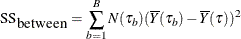
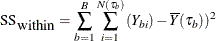
For continuous response variables, the worth is based on the F test for the null hypothesis that the means of the response values are identical across the child nodes. The test statistic is
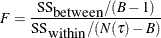
where
Available for both categorical and continuous response variables:
-
CHAID criterion
For categorical and continuous response variables, CHAID is an approach first described by Kass (1980) that regards every possible split as representing a test. CHAID tests the hypothesis of no association between the values of the response (target) and the branches of a node. The Bonferroni adjusted probability is defined as m
 , where is the significance level of a test and m is the number of independent tests.
For categorical response variables, the HPSPLIT procedure also provides the FastCHAID criterion, which is a special case of CHAID. FastCHAID is faster to compute because it prioritizes the possible splits by sorting them according to the response variable.