The HPSPLIT Procedure

Building a Decision Tree
Algorithms for building a decision tree use the training data to split the predictor space (the set of all possible combinations of values of the predictor variables) into nonoverlapping regions. These regions correspond to the terminal nodes of the tree, which are also known as leaves.
Each region is described by a set of rules, and these rules are used to assign a new observation to a particular region. In the case of a classification tree, the predicted value for this observation is the most commonly occurring level of the response variable in that region; in the case of a regression tree, the predicted value is the mean of the values of the response variables in that region.
The splitting is done by recursive partitioning, starting with all the observations, which are represented by the node at the top of the tree. The algorithm splits this parent node into two or more child nodes in such a way that the responses within each child region are as similar as possible. The splitting process is then repeated for each of the child nodes, and the recursion continues until a stopping criterion is satisfied and the tree is fully built.
At each step, the split is determined by finding a best predictor variable and a best cutpoint (or set of cutpoints) that assign the observations in the parent node to the child nodes. The sections Splitting Criteria and Splitting Strategy provide details about the splitting methods available in the HPSPLIT procedure.
To illustrate the process, consider the first two splits for the classification tree in Example 61.4: Creating a Binary Classification Tree with Validation Data, which is shown in Figure 61.11.
Figure 61.11: First Two Splits for Hmeq Data Set
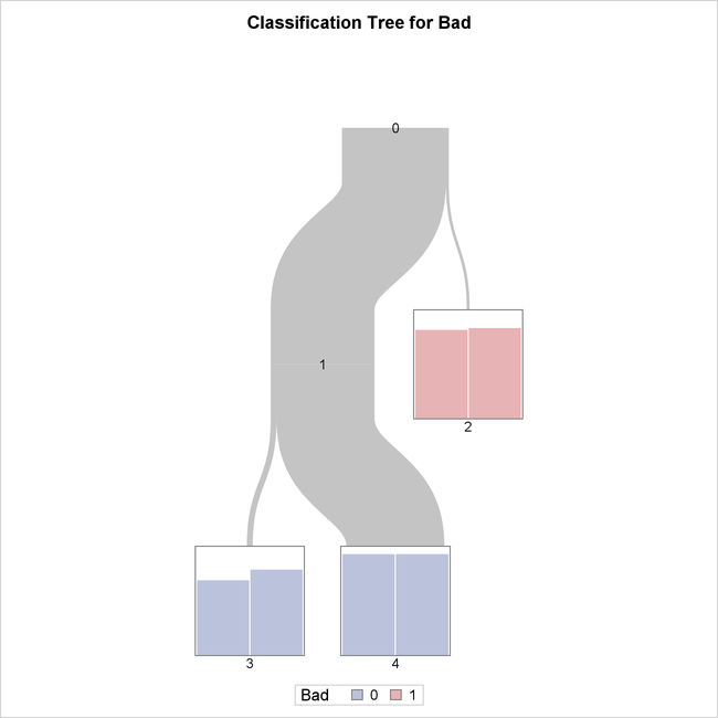
All 2,352 observations in the data are initially assigned to Node 0 at the top of the tree, which represents the entire predictor
space. The algorithm then splits this space into two nonoverlapping regions, represented by Node 1 and Node 2. Observations
with Debtinc < 48.8434 or with missing values of Debtinc are assigned to Node 1, and observations with Debtinc > 48.8434 are assigned to Node 2. Here the best variable, Debtinc, and the best cutpoint, 48.8434, are chosen to maximize the reduction in entropy as a measure of node impurity.
Next, the algorithm splits the region that is represented by Node 1 into two nonoverlapping regions, represented by Node 3
and Node 4. Observations with values of the categorical predictor variable Delinq equal to 2, 3, 4, 5, 6, or 7 are assigned to Node 3, and observations with Delinq equal to 0, 1, 8, 9, 10, 11, 12, 14, 15, or missing are assigned to Node 4. Note that the levels of Delinq in Node 4 are not adjacent to each other. Here the best variable, Delinq, and the values 2, 3, 4, 5, 6, and 7 are chosen to maximize the reduction in entropy.
Figure 61.12: Scatter Plot of the Predictor Space for the First Split
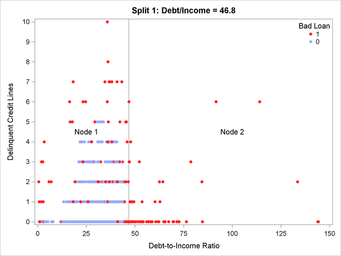
Figure 61.13: Scatter Plot of the Predictor Space for the Second Split
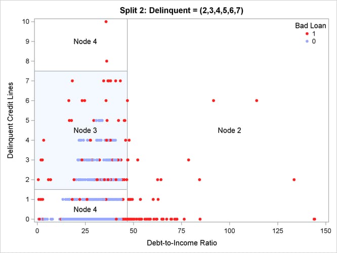
The tree that is defined by these two splits has three leaf (terminal) nodes, which are Nodes 2, 3, and 4 in Figure 61.13. Figure 61.12 and Figure 61.13 present scatter plots of the predictor space for these two splits one at a time. Notice in Figure 61.12 that the first split in Debt-to-Income Ratio divides the entire predictor space into Node 1 and Node 2, represented by two rectangular regions that have different ratios
of events to nonevents for the response variable. In a similar way, notice in Figure 61.13 that the second split in Delinquent Credit Lines divides Node 1 into Node 3 and 4, which have different ratios of events to nonevents for the response variable. Also note
that several observations have the same values for Debtinc or Delinq, giving the perception of a scatter plot that has fewer observations than there actually are.
For example, Node 4 has a very high proportion of observations for which Bad is equal to 0. In contrast, Bad is equal to 1 for all the observations in Node 2.
This example illustrates recursive binary splitting in which each parent node is split into two child nodes. By default, the HPSPLIT procedure finds two-way splits when building regression trees, and it finds k-way splits when building classification trees, where k is the number of levels of the categorical response variable. You can use the MAXBRANCH= option to specify the k-way splits of your tree.