HISTOGRAM Statement: CAPABILITY Procedure

Example 5.9 Fitting Lognormal, Weibull, and Gamma Curves
[See CAPCURV in the SAS/QC Sample Library]To find an appropriate model for a process distribution, you should consider curves from several distribution families. As shown in this example, you can use the HISTOGRAM statement to fit more than one type of distribution and display the density curves on the same histogram.
The gap between two plates is measured (in cm) for each of 50 welded assemblies selected at random from the output of a welding process assumed to be in statistical control. The lower and upper specification limits for the gap are 0.3 cm and 0.8 cm, respectively. The measurements are saved in a data set named Plates.
data Plates;
   label Gap='Plate Gap in cm';
   input Gap @@;
   datalines;
0.746  0.357  0.376  0.327  0.485 1.741  0.241  0.777  0.768  0.409
0.252  0.512  0.534  1.656  0.742 0.378  0.714  1.121  0.597  0.231
0.541  0.805  0.682  0.418  0.506 0.501  0.247  0.922  0.880  0.344
0.519  1.302  0.275  0.601  0.388 0.450  0.845  0.319  0.486  0.529
1.547  0.690  0.676  0.314  0.736 0.643  0.483  0.352  0.636  1.080
;
The following statements fit three distributions (lognormal, Weibull, and gamma) and display their density curves on a single histogram:
ods graphics on;
proc capability data=Plates;
   var Gap;
   specs  lsl = 0.3 usl = 0.8;
   histogram /
       midpoints=0.2 to 1.8 by 0.2
       lognormal
       weibull
       gamma
       nospeclegend;
   inset n mean(5.3) std='Std Dev'(5.3) skewness(5.3)
          / pos = ne  header = 'Summary Statistics';
run;
The LOGNORMAL, WEIBULL, and GAMMA options superimpose fitted curves on the histogram in Output 5.9.1. Note that a threshold parameter  is assumed for each curve. In applications where the threshold is not zero, you can specify
  with the THETA= option.
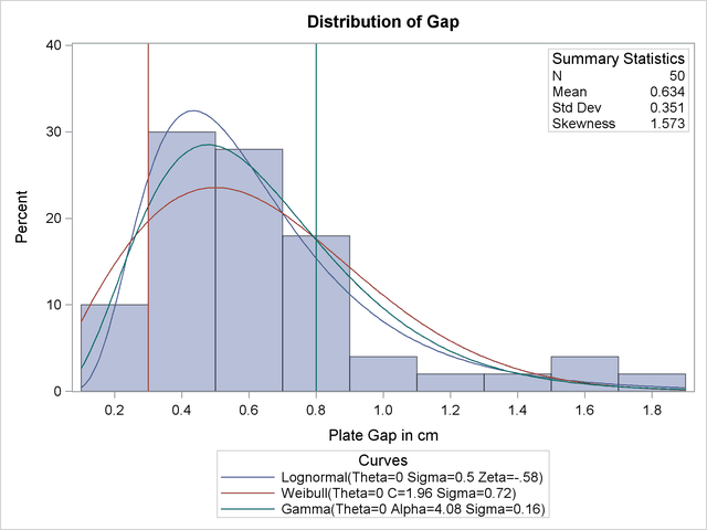
The LOGNORMAL, WEIBULL, and GAMMA options also produce the summaries for the fitted distributions shown in Output 5.9.2, Output 5.9.3, and Output 5.9.4.
| Parameters for Lognormal Distribution | ||
|---|---|---|
| Parameter | Symbol | Estimate |
| Threshold | Theta | 0 |
| Scale | Zeta | -0.58375 |
| Shape | Sigma | 0.499546 |
| Mean | 0.631932 | |
| Std Dev | 0.336436 | |
| Goodness-of-Fit Tests for Lognormal Distribution | |||||
|---|---|---|---|---|---|
| Test | Statistic | DF | p Value | ||
| Kolmogorov-Smirnov | D | 0.06441431 | Pr > D | >0.150 | |
| Cramer-von Mises | W-Sq | 0.02823022 | Pr > W-Sq | >0.500 | |
| Anderson-Darling | A-Sq | 0.24308402 | Pr > A-Sq | >0.500 | |
| Chi-Square | Chi-Sq | 7.51762213 | 6 | Pr > Chi-Sq | 0.276 |
| Percent Outside Specifications for Lognormal Distribution | |||
|---|---|---|---|
| Lower Limit | Upper Limit | ||
| LSL | 0.300000 | USL | 0.800000 |
| Obs Pct < LSL | 10.000000 | Obs Pct > USL | 20.000000 |
| Est Pct < LSL | 10.719540 | Est Pct > USL | 23.519008 |
| Quantiles for Lognormal Distribution | ||
|---|---|---|
| Percent | Quantile | |
| Observed | Estimated | |
| 1.0 | 0.23100 | 0.17449 |
| 5.0 | 0.24700 | 0.24526 |
| 10.0 | 0.29450 | 0.29407 |
| 25.0 | 0.37800 | 0.39825 |
| 50.0 | 0.53150 | 0.55780 |
| 75.0 | 0.74600 | 0.78129 |
| 90.0 | 1.10050 | 1.05807 |
| 95.0 | 1.54700 | 1.26862 |
| 99.0 | 1.74100 | 1.78313 |
Output 5.9.2 provides four goodness-of-fit tests for the lognormal distribution: the chi-square test and three tests based on the EDF (Anderson-Darling, Cramer-von Mises, and Kolmogorov-Smirnov). See Chi-Square Goodness-of-Fit Test and EDF Goodness-of-Fit Tests for more information. The EDF tests are superior to the chi-square test because they are not dependent on the set of midpoints used for the histogram.
At the  significance level, all four tests support the conclusion that the two-parameter lognormal distribution with scale parameter
  , and shape parameter
  provides a good model for the distribution of plate gaps.
| Parameters for Weibull Distribution | ||
|---|---|---|
| Parameter | Symbol | Estimate |
| Threshold | Theta | 0 |
| Scale | Sigma | 0.719208 |
| Shape | C | 1.961159 |
| Mean | 0.637641 | |
| Std Dev | 0.339248 | |
| Goodness-of-Fit Tests for Weibull Distribution | |||||
|---|---|---|---|---|---|
| Test | Statistic | DF | p Value | ||
| Cramer-von Mises | W-Sq | 0.1593728 | Pr > W-Sq | 0.016 | |
| Anderson-Darling | A-Sq | 1.1569354 | Pr > A-Sq | <0.010 | |
| Chi-Square | Chi-Sq | 15.0252996 | 6 | Pr > Chi-Sq | 0.020 |
| Percent Outside Specifications for Weibull Distribution | |||
|---|---|---|---|
| Lower Limit | Upper Limit | ||
| LSL | 0.300000 | USL | 0.800000 |
| Obs Pct < LSL | 10.000000 | Obs Pct > USL | 20.000000 |
| Est Pct < LSL | 16.473319 | Est Pct > USL | 29.165543 |
| Quantiles for Weibull Distribution | ||
|---|---|---|
| Percent | Quantile | |
| Observed | Estimated | |
| 1.0 | 0.23100 | 0.06889 |
| 5.0 | 0.24700 | 0.15817 |
| 10.0 | 0.29450 | 0.22831 |
| 25.0 | 0.37800 | 0.38102 |
| 50.0 | 0.53150 | 0.59661 |
| 75.0 | 0.74600 | 0.84955 |
| 90.0 | 1.10050 | 1.10040 |
| 95.0 | 1.54700 | 1.25842 |
| 99.0 | 1.74100 | 1.56691 |
Output 5.9.3 provides two EDF goodness-of-fit tests for the Weibull distribution: the Anderson-Darling and the Cramer-von Mises tests. (See Table 5.23 for a complete list of the EDF tests available in the HISTOGRAM statement.) The probability values for the chi-square and EDF tests are all less than  , indicating that the data do not support a Weibull model.
| Parameters for Gamma Distribution | ||
|---|---|---|
| Parameter | Symbol | Estimate |
| Threshold | Theta | 0 |
| Scale | Sigma | 0.155198 |
| Shape | Alpha | 4.082646 |
| Mean | 0.63362 | |
| Std Dev | 0.313587 | |
| Goodness-of-Fit Tests for Gamma Distribution | |||||
|---|---|---|---|---|---|
| Test | Statistic | DF | p Value | ||
| Kolmogorov-Smirnov | D | 0.0969533 | Pr > D | >0.250 | |
| Cramer-von Mises | W-Sq | 0.0739847 | Pr > W-Sq | >0.250 | |
| Anderson-Darling | A-Sq | 0.5810661 | Pr > A-Sq | 0.137 | |
| Chi-Square | Chi-Sq | 12.3075959 | 6 | Pr > Chi-Sq | 0.055 |
| Percent Outside Specifications for Gamma Distribution | |||
|---|---|---|---|
| Lower Limit | Upper Limit | ||
| LSL | 0.300000 | USL | 0.800000 |
| Obs Pct < LSL | 10.000000 | Obs Pct > USL | 20.000000 |
| Est Pct < LSL | 12.111039 | Est Pct > USL | 25.696522 |
| Quantiles for Gamma Distribution | ||
|---|---|---|
| Percent | Quantile | |
| Observed | Estimated | |
| 1.0 | 0.23100 | 0.13326 |
| 5.0 | 0.24700 | 0.21951 |
| 10.0 | 0.29450 | 0.27938 |
| 25.0 | 0.37800 | 0.40404 |
| 50.0 | 0.53150 | 0.58271 |
| 75.0 | 0.74600 | 0.80804 |
| 90.0 | 1.10050 | 1.05392 |
| 95.0 | 1.54700 | 1.22160 |
| 99.0 | 1.74100 | 1.57939 |
Output 5.9.4 provides four goodness-of-fit tests for the gamma distribution. The probability value for the chi-square test is less than , indicating that the data do not support a gamma model.
Based on this analysis, the fitted lognormal distribution is the best model for the distribution of plate gaps. You can use this distribution to calculate useful quantities. For instance, you can compute the probability that the gap of a randomly sampled plate exceeds the upper specification limit, as follows:
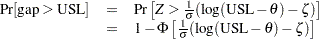 |
where  has a standard normal distribution, and
  is the standard normal cumulative distribution function. Note that can be computed with the DATA step function PROBNORM. In this example, USL
  and
and 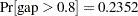 . This value is expressed as a percent (Est Pct > USL) in Output 5.9.2.