HISTOGRAM Statement: CAPABILITY Procedure

Formulas for Fitted Curves
The following sections provide information about the families of parametric distributions that you can fit with the HISTOGRAM statement. Properties of these distributions are discussed by Johnson, Kotz, and Balakrishnan (1994) and Johnson, Kotz, and Balakrishnan (1995).
Beta Distribution
The fitted density function is
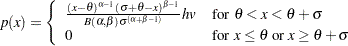 |
where 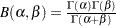 and
and  lower threshold parameter (lower endpoint parameter)
  scale parameter
 shape parameter
 shape parameter
 width of histogram interval
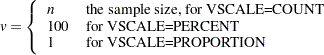
  vertical scaling factor, and
 |
Note: This notation is consistent with that of other distributions that you can fit with the HISTOGRAM statement. However, many texts, including Johnson, Kotz, and Balakrishnan (1995), write the beta density function as
 |
The two notations are related as follows: 


The range of the beta distribution is bounded below by a threshold parameter and above by  . If you specify a fitted beta curve by using the BETA option,
  must be less than the minimum data value, and
  must be greater than the maximum data value. You can specify and
  with the THETA= and SIGMA= beta-options in parentheses after the keyword BETA. By default,
  and
and  . If you specify THETA=EST and SIGMA=EST, maximum likelihood estimates are computed for and .
In addition, you can specify  and
and  with the ALPHA= and BETA= beta-options, respectively. By default, the procedure calculates maximum likelihood estimates for and . For example, to fit a beta density curve to a set of data bounded below by 32 and above by 212 with maximum likelihood estimates for and , use the following statement:
histogram length / beta(theta=32 sigma=180);
The beta distributions are also referred to as Pearson Type I or II distributions. These include the power-function distribution ( ), the arc-sine distribution (
 ), and the generalized arc-sine distributions (
 ,
,  ).
).
You can use the DATA step function BETAINV to compute beta quantiles and the DATA step function PROBBETA to compute beta probabilities.
Exponential Distribution
The fitted density function is
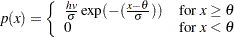 |
where threshold parameter scale parameter width of histogram interval vertical scaling factor, and
|
The threshold parameter must be less than or equal to the minimum data value. You can specify with the THRESHOLD= exponential-option. By default, . If you specify THETA=EST, a maximum likelihood estimate is computed for . In addition, you can specify with the SCALE= exponential-option. By default, the procedure calculates a maximum likelihood estimate for . Note that some authors define the scale parameter as  .
.
The exponential distribution is a special case of both the gamma distribution (with  ) and the Weibull distribution (with
  ). A related distribution is the extreme value distribution. If
  has an exponential distribution, then
  has an extreme value distribution.
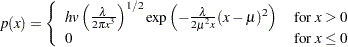
Gamma Distribution
The fitted density function is
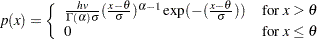 |
where threshold parameter scale parameter shape parameter width of histogram interval vertical scaling factor, and
|
The threshold parameter must be less than the minimum data value. You can specify with the THRESHOLD= gamma-option. By default, . If you specify THETA=EST, a maximum likelihood estimate is computed for . In addition, you can specify and with the SCALE= and ALPHA= gamma-options. By default, the procedure calculates maximum likelihood estimates for and .
The gamma distributions are also referred to as Pearson Type III distributions, and they include the chi-square, exponential, and Erlang distributions. The probability density function for the chi-square distribution is
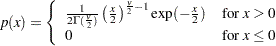 |
Notice that this is a gamma distribution with  ,
,  , and . The exponential distribution is a gamma distribution with , and the Erlang distribution is a gamma distribution with being a positive integer. A related distribution is the Rayleigh distribution. If
  where the
  ’s are independent
  variables, then
  is distributed with a
  distribution having a probability density function of
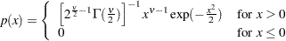 |
If  , the preceding distribution is referred to as the Rayleigh distribution.
You can use the DATA step function GAMINV to compute gamma quantiles and the DATA step function PROBGAM to compute gamma probabilities.
Gumbel Distribution
The fitted density function is
 |
where  location parameter scale parameter width of histogram interval vertical scaling factor, and
|
You can specify  and with the MU= and SIGMA= Gumbel-options, respectively. By default, the procedure calculates maximum likelihood estimates for these parameters.
Note: The Gumbel distribution is also referred to as Type 1 extreme value distribution.
Note: The random variable has Gumbel (Type 1 extreme value) distribution if and only if  has Weibull distribution and
  has standard exponential distribution.
Inverse Gaussian Distribution
The fitted density function is
 |
where location parameter 
 shape parameter
  width of histogram interval vertical scaling factor, and
|
The location parameter has to be greater then zero. You can specify with the MU= iGauss-option. In addition, you can specify shape parameter  with the LAMBDA= iGauss-option. By default, the procedure uses the sample mean for and calculates a maximum likelihood estimate for .
Note: The special case where  and
and  corresponds to the Wald distribution.
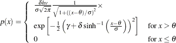
Lognormal Distribution
The fitted density function is
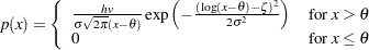 |
where threshold parameter  scale parameter
  shape parameter width of histogram interval vertical scaling factor, and
|
The threshold parameter must be less than the minimum data value. You can specify with the THRESHOLD= lognormal-option. By default, . If you specify THETA=EST, a maximum likelihood estimate is computed for . You can specify  and with the SCALE= and SHAPE= lognormal-options, respectively. By default, the procedure calculates maximum likelihood estimates for these parameters.
Note: The lognormal distribution is also referred to as the  distribution in the Johnson system of distributions.
Note: This book uses to denote the shape parameter of the lognormal distribution, whereas is used to denote the scale parameter of the beta, exponential, gamma, Gumbel, inverse Gaussian, normal, generalized Pareto, power function, Rayleigh, and Weibull distributions. The use of to denote the lognormal shape parameter is based on the fact that 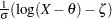 has a standard normal distribution if is lognormally distributed.
Normal Distribution
The fitted density function is
 |
where mean standard deviation width of histogram interval vertical scaling factor, and
|
You can specify and with the MU= and SIGMA= normal-options, respectively. By default, the procedure estimates with the sample mean and with the sample standard deviation.
You can use the DATA step function PROBIT to compute normal quantiles and the DATA step function PROBNORM to compute probabilities.
Note: The normal distribution is also referred to as the  distribution in the Johnson system of distributions.
Generalized Pareto Distribution
The fitted density function is
 |
where threshold parameter scale parameter shape parameter width of histogram interval vertical scaling factor, and
|
The support of the distribution is  for
for  and
and  for
for  .
.
Note: Special cases of the generalized Pareto distribution with  and correspond respectively to the exponential distribution with mean and uniform distribution on the interval
  .
.
The threshold parameter must be less than the minimum data value. You can specify with the THETA= Pareto-option. By default, . You can also specify and with the ALPHA= and SIGMA= Pareto-options,respectively. By default, the procedure calculates maximum likelihood estimates for these parameters.
Note: Maximum likelihood estimation of the parameters works well if  , but not otherwise. In this case the estimators are asymptotically normal and asymptotically efficient. The asymptotic normal distribution of the maximum likelihood estimates has mean
  and variance-covariance matrix
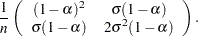 |
Note: If no local minimum found in the space
 |
there is no maximum likelihood estimator. More details on how to find maximum likelihood estimators and suggested algorithm can be found in Grimshaw(1993).
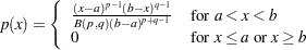
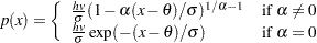
Power Function Distribution
The fitted density function is
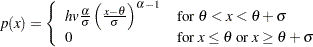 |
where lower threshold parameter (lower endpoint parameter) scale parameter shape parameter width of histogram interval vertical scaling factor, and
|
Note: This notation is consistent with that of other distributions that you can fit with the HISTOGRAM statement. However, many texts, including Johnson, Kotz, and Balakrishnan (1995), write the density function of power function distribution as
 |
The two parameterizations are related as follows:
Note: The family of power function distributions is a subclass of beta distribution with density function
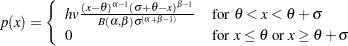 |
where with parameter  . Therefore, all properties and estimation procedures of beta distribution apply.
The range of the power function distribution is bounded below by a threshold parameter and above by . If you specify a fitted power function curve by using the POWER option, must be less than the minimum data value and must be greater than the maximum data value. You can specify and with the THETA= and SIGMA= power-options in parentheses after the keyword POWER. By default, and . If you specify THETA=EST and SIGMA=EST, maximum likelihood estimates are computed for and . However, three-parameter maximum likelihood estimation does not always converge.
In addition, you can specify with the ALPHA= power-option. By default, the procedure calculates a maximum likelihood estimate for . For example, to fit a power function density curve to a set of data bounded below by 32 and above by 212 with maximum likelihood estimate for , use the following statement:
histogram Length / power(theta=32 sigma=180);
Rayleigh Distribution
The fitted density function is
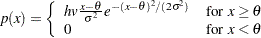 |
where lower threshold parameter (lower endpoint parameter) scale parameter width of histogram interval vertical scaling factor, and
|
Note: The Rayleigh distribution is a Weibull distribution with density function
 |
and with shape parameter  and scale parameter
  .
.
The threshold parameter must be less than the minimum data value. You can specify with the THETA= Rayleigh-option. By default, . In addition you can specify with the SIGMA= Rayleigh-option. By default, the procedure calculates maximum likelihood estimate for .
For example, to fit a Rayleigh density curve to a set of data bounded below by 32 with maximum likelihood estimate for , use the following statement:
histogram Length / rayleigh(theta=32);
Johnson  Distribution
The fitted density function is
 |
where threshold parameter  scale parameter
 shape parameter
 shape parameter
  width of histogram interval vertical scaling factor, and
|
The distribution is bounded below by the parameter and above by the value . The parameter must be less than the minimum data value. You can specify with the THETA= -option, or you can request that be estimated with the THETA = EST -option. The default value for is zero. The sum must be greater than the maximum data value. The default value for is one. You can specify with the SIGMA= -option, or you can request that be estimated with the SIGMA = EST -option.
By default, the method of percentiles given by Slifker and Shapiro (1980) is used to estimate the parameters. This method is based on four data percentiles, denoted by  ,
,  ,
,  , and
, and  , which correspond to the four equally spaced percentiles of a standard normal distribution, denoted by
  ,
,  ,
,  , and
, and  , under the transformation
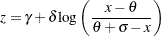 |
The default value of is 0.524. The results of the fit are dependent on the choice of , and you can specify other values with the FITINTERVAL= option (specified in parentheses after the SB option). If you use the method of percentiles, you should select a value of that corresponds to percentiles which are critical to your application.
The following values are computed from the data percentiles:
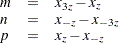 |
It was demonstrated by Slifker and Shapiro (1980) that
 |
A tolerance interval around one is used to discriminate among the three families with this ratio criterion. You can specify the tolerance with the FITTOLERANCE= option (specified in parentheses after the SB option). The default tolerance is 0.01. Assuming that the criterion satisfies the inequality
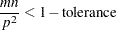 |
the parameters of the distribution are computed using the explicit formulas derived by Slifker and Shapiro (1980).
If you specify FITMETHOD = MOMENTS (in parentheses after the SB option) the method of moments is used to estimate the parameters. If you specify FITMETHOD = MLE (in parentheses after the SB option) the method of maximum likelihood is used to estimate the parameters. Note that maximum likelihood estimates may not always exist. Refer to Bowman and Shenton (1983) for discussion of methods for fitting Johnson distributions.
Johnson  Distribution
The fitted density function is
 |
where location parameter scale parameter shape parameter shape parameter width of histogram interval vertical scaling factor, and
|
You can specify the parameters with the THETA=, SIGMA=, DELTA=, and GAMMA= -options, which are enclosed in parentheses after the SU option. If you do not specify these parameters, they are estimated.
By default, the method of percentiles given by Slifker and Shapiro (1980) is used to estimate the parameters. This method is based on four data percentiles, denoted by , , , and , which correspond to the four equally spaced percentiles of a standard normal distribution, denoted by , , , and , under the transformation
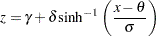 |
The default value of is 0.524. The results of the fit are dependent on the choice of , and you can specify other values with the FITINTERVAL= option (specified in parentheses after the SB option). If you use the method of percentiles, you should select a value of that corresponds to percentiles which are critical to your application. You can specify the value of with the FITINTERVAL= option (specified in parentheses after the SU option).
The following values are computed from the data percentiles:
|
It was demonstrated by Slifker and Shapiro (1980) that
|
A tolerance interval around one is used to discriminate among the three families with this ratio criterion. You can specify the tolerance with the FITTOLERANCE= option (specified in parentheses after the SU option). The default tolerance is 0.01. Assuming that the criterion satisfies the inequality
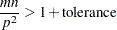 |
the parameters of the distribution are computed using the explicit formulas derived by Slifker and Shapiro (1980).
If you specify FITMETHOD = MOMENTS (in parentheses after the SU option) the method of moments is used to estimate the parameters. If you specify FITMETHOD = MLE (in parentheses after the SU option) the method of maximum likelihood is used to estimate the parameters. Note that maximum likelihood estimates may not always exist. Refer to Bowman and Shenton (1983) for discussion of methods for fitting Johnson distributions.
Weibull Distribution
The fitted density function is
 |
where threshold parameter scale parameter  shape parameter
  width of histogram interval vertical scaling factor, and
|
The threshold parameter must be less than the minimum data value. You can specify with the THRESHOLD= Weibull-option. By default, . If you specify THETA=EST, a maximum likelihood estimate is computed for . You can specify and  with the SCALE= and SHAPE= Weibull-options, respectively. By default, the procedure calculates maximum likelihood estimates for and .
The exponential distribution is a special case of the Weibull distribution where .