The OPTMODEL Procedure

Getting Started: OPTMODEL Procedure

Subsections:

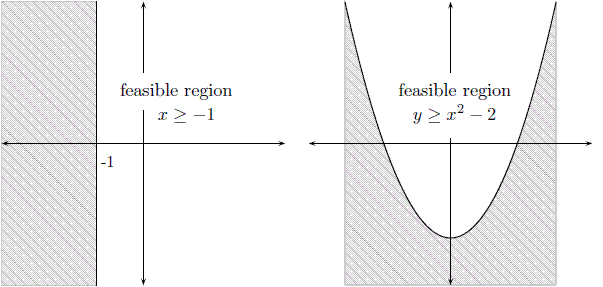
Optimization or mathematical programming is a search for a maximum or minimum of an objective function (also called a cost function), where search variables are restricted to particular constraints. Constraints are said to define a feasible region (see Figure 5.1).

Figure 5.1: Examples of Feasible Regions

A more rigorous general formulation of such problems is as follows.

Let

$f:S\rightarrow \mathbb {R}$

be a real-valued function. Find $x^*$ such that

$x^* \in S$
$f(x^*) \leq f(x), \quad \forall x \in S$

Note that the formulation is for the minimum of f and that the maximum of f is simply the negation of the minimum of $-f$ .

Here, function f is the objective function, and the variable in the objective function is called the optimization variable (or decision variable). S is the feasible region. Typically S is a subset of the Euclidean space $\mathbb {R}^ n$ specified by the set of constraints, which are often a set of equalities (=) or inequalities ( $\leq , \geq$ ) that every element in S is required to satisfy simultaneously. For the special case where $S=\mathbb {R}^ n$ , the problem is an unconstrained optimization. An element x of S is called a feasible solution to the optimization problem, and the value $f(x)$ is called the objective value. A feasible solution $x^*$ that minimizes the objective function is called an optimal solution to the optimization problem, and the corresponding objective value is called the optimal value.

In mathematics, special notation is used to denote an optimization problem. Generally, you can write an optimization problem as follows:

$\begin{array}{rl} \displaystyle \mathop {\textrm{minimize}}& f(x)\\ \textrm{subject to}& x \in S \end{array}$

Normally, an empty body of constraint (the part after "subject to") implies that the optimization is unconstrained (that is, the feasible region is the whole space $\mathbb {R}^ n$ ). The optimal solution ( $x^*$ ) is denoted as

$x^*=\mathop {\mr{argmin}}_{x \in S}f(x)$

The optimal value ( $f(x^*)$ ) is denoted as

$f(x^*)=\mathop {\min }_{x\in S}f(x)$

Optimization problems can be classified by the forms (linear, quadratic, nonlinear, and so on) of the functions in the objective and constraints. For example, a problem is said to be linearly constrained if the functions in the constraints are linear. A linear programming problem is a linearly constrained problem with a linear objective function. A nonlinear programming problem occurs where some function in the objective or constraints is nonlinear, and so on.