The OPTMODEL Procedure
- Overview
-
Getting Started

-
Syntax
-
DetailsNamed ParametersIndexingTypesNamesParametersExpressionsIdentifier ExpressionsFunction ExpressionsIndex SetsOPTMODEL Expression ExtensionsConditions of OptimalityData Set Input/OutputControl FlowFormatted OutputODS Table and Variable NamesConstraintsSuffixesInteger Variable SuffixesDual ValuesReduced CostsPresolverModel UpdateMultiple SubproblemsMultiple SolutionsProblem SymbolsOPTMODEL OptionsAutomatic DifferentiationConversionsFCMP RoutinesMore on Index SetsThreaded and Distributed ProcessingMacro Variable _OROPTMODEL_Rewriting PROC NLP Models for PROC OPTMODEL
-
Examples
- References
Conditions of Optimality
Linear Programming
A standard linear program has the following formulation:
![\[ \begin{array}{rl} \displaystyle \mathop {\textrm{minimize}}& \mathbf{c}^{T} \mathbf{x} \\ \textrm{subject to}& \mathbf{A} \mathbf{x} \ge \mathbf{b} \\ & \mathbf{x} \ge 0 \end{array} \]](images/ormpug_optmodel0051.png)
where
|
|
|
|
is the vector of decision variables |
|
|
|
|
is the matrix of constraints |
|
|
|
|
is the vector of objective function coefficients |
|
|
|
|
is the vector of constraints right-hand sides (RHS) |


This formulation is called the primal problem. The corresponding dual problem (see the section Dual Values) is
![\[ \begin{array}{rl} \displaystyle \mathop {\textrm{maximize}}& \mathbf{b}^{T} \mathbf{y} \\ \textrm{subject to}& \mathbf{A}^{T} \mathbf{y} \le \mathbf{c} \\ & \mathbf{y} \ge 0 \end{array} \]](images/ormpug_optmodel0061.png)
where  is the vector of dual variables.
The vectors  and
and  are optimal to the primal and dual problems, respectively, only if there exist primal slack variables
  and dual slack variables
  such that the following Karush-Kuhn-Tucker (KKT) conditions are satisfied:
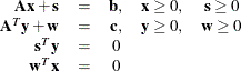
The first line of equations defines primal feasibility, the second line of equations defines dual feasibility, and the last two equations are called the complementary slackness conditions.
Nonlinear Programming
To facilitate discussion of optimality conditions in nonlinear programming, you write the general form of nonlinear optimization
problems by grouping the equality constraints and inequality constraints. You also write all the general nonlinear inequality
constraints and bound constraints in one form as " " inequality constraints. Thus, you have the following formulation:
![\[ \begin{array}{lll} \displaystyle \mathop {\textrm{minimize}}_{x\in {\mathbb R}^ n} & f(x) \\ \textrm{subject to}& c_ i(x) = 0, & i \in {\mathcal E} \\ & c_ i(x) \ge 0, & i \in {\mathcal I} \end{array} \]](images/ormpug_optmodel0068.png)
where  is the set of indices of the equality constraints,
  is the set of indices of the inequality constraints, and
  .
.
A point x is feasible if it satisfies all the constraints  and
and  .
The feasible region
.
The feasible region  consists of all the feasible points. In unconstrained cases, the feasible region is the entire
  space.
A feasible point  is a local solution of the problem if there exists a neighborhood
  of such that
![\[ f(x)\ge f(x^*)\; \; {\mathrm for\ all\ } x\in {\mathcal N}\cap {\mathcal F} \]](images/ormpug_optmodel0077.png)
Further, a feasible point is a strict local solution if strict inequality holds in the preceding case; that is,
![\[ f(x) > f(x^*)\; \; {\mathrm for\ all\ } x\in {\mathcal N}\cap {\mathcal F} \]](images/ormpug_optmodel0078.png)
A feasible point is a global solution of the problem if no point in has a smaller function value than  ); that is,
![\[ f(x)\ge f(x^*)\; \; {\mathrm for \ all \ } x\in {\mathcal F} \]](images/ormpug_optmodel0080.png)
Unconstrained Optimization
The following conditions hold true for unconstrained optimization problems:
-
First-order necessary conditions: If
is a local solution and  is continuously differentiable in some neighborhood of , then
![\[ \nabla \! f(x^*) = 0 \]](images/ormpug_optmodel0081.png)
-
Second-order necessary conditions: If
is a local solution and is twice continuously differentiable in some neighborhood of , then  is positive semidefinite.
-
Second-order sufficient conditions: If
is twice continuously differentiable in some neighborhood of ,  , and is positive definite, then is a strict local solution.
Constrained Optimization
For constrained optimization problems, the Lagrangian function is defined as follows:
![\[ L(x,\lambda ) = f(x) - \sum _{i\in {\mathcal E}\cup {\mathcal I}} \lambda _ i c_ i(x) \]](images/ormpug_optmodel0084.png)
where  , are called Lagrange multipliers.
 is used to denote the gradient of the Lagrangian function with respect to x, and
  is used to denote the Hessian of the Lagrangian function with respect to x. The active set at a feasible point x is defined as
![\[ {\mathcal A}(x)={\mathcal E}\cup \{ i\in {\mathcal I}: c_ i(x)=0\} \]](images/ormpug_optmodel0088.png)
You also need the following definition before you can state the first-order and second-order necessary conditions:
-
Linear independence constraint qualification and regular point: A point x is said to satisfy the linear independence constraint qualification if the gradients of active constraints
![\[ \nabla \! c_ i(x),\quad i\in {\mathcal A}(x) \]](images/ormpug_optmodel0089.png)
are linearly independent. Such a point x is called a regular point.
You now state the theorems that are essential in the analysis and design of algorithms for constrained optimization:
-
First-order necessary conditions: Suppose that
is a local minimum and also a regular point. If and  , are continuously differentiable, there exist Lagrange multipliers
  such that the following conditions hold:
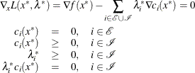
The preceding conditions are often known as the Karush-Kuhn-Tucker conditions, or KKT conditions for short.
-
Second-order necessary conditions: Suppose that
is a local minimum and also a regular point. Let  be the Lagrange multipliers that satisfy the KKT conditions. If and
  , are twice continuously differentiable, the following conditions hold:
![\[ z^ T \nabla _{\! x}^2 L(x^*,\lambda ^*)z \ge 0 \]](images/ormpug_optmodel0095.png)
for all
 that satisfy
![\[ \nabla \! c_ i(x^*)^ Tz = 0,\quad i\in {\mathcal A}(x^{*}) \]](images/ormpug_optmodel0097.png)
-
Second-order sufficient conditions: Suppose there exist a point
and some Lagrange multipliers such that the KKT conditions are satisfied. If
![\[ z^ T \nabla _{\! x}^2 L(x^*,\lambda ^*)z > 0 \]](images/ormpug_optmodel0098.png)
for all
that satisfy
![\[ \nabla \! c_ i(x^*)^ Tz = 0,\quad i\in {\mathcal A}(x^*) \]](images/ormpug_optmodel0099.png)
then
is a strict local solution.
Note that the set of all such z’s forms the null space of the matrix
![$\left[\nabla \! c_ i(x^*)^ T \right]_{i\in {\mathcal A}(x^{*})}$](images/ormpug_optmodel0100.png) . Thus, you can search for strict local solutions by numerically checking the Hessian of the Lagrangian function projected
onto the null space. For a rigorous treatment of the optimality conditions, see Fletcher (1987) and Nocedal and Wright (1999).
. Thus, you can search for strict local solutions by numerically checking the Hessian of the Lagrangian function projected
onto the null space. For a rigorous treatment of the optimality conditions, see Fletcher (1987) and Nocedal and Wright (1999).