The PANEL Procedure
- Overview
- Getting Started
-
Syntax

-
DetailsSpecifying the Input DataSpecifying the Regression ModelUnbalanced DataMissing ValuesComputational ResourcesRestricted EstimatesNotationOne-Way Fixed-Effects ModelTwo-Way Fixed-Effects ModelBalanced PanelsUnbalanced PanelsFirst-Differenced Methods for One-Way and Two-Way ModelsBetween EstimatorsPooled EstimatorOne-Way Random-Effects ModelTwo-Way Random-Effects ModelHausman-Taylor EstimationAmemiya-MaCurdy EstimationParks Method (Autoregressive Model)Da Silva Method (Variance-Component Moving Average Model)Dynamic Panel EstimatorsLinear Hypothesis TestingHeteroscedasticity-Corrected Covariance MatricesHeteroscedasticity- and Autocorrelation-Consistent Covariance MatricesR-SquareSpecification TestsPanel Data Poolability TestPanel Data Cross-Sectional Dependence TestPanel Data Unit Root TestsLagrange Multiplier (LM) Tests for Cross-Sectional and Time EffectsTests for Serial Correlation and Cross-Sectional EffectsTroubleshootingCreating ODS GraphicsOUTPUT OUT= Data SetOUTEST= Data SetOUTTRANS= Data SetPrinted OutputODS Table Names
-
Examples
- References
Lagrange Multiplier (LM) Tests for Cross-Sectional and Time Effects
For random one-way and two-way error component models, the Lagrange multiplier test for the existence of cross-sectional or time effects or both is based on the residuals from the restricted model (that is, the pooled model). For more information about the Breusch-Pagan LM test, see the section Specification Tests.
The Breusch-Pagan LM test is two-sided when the variance components are nonnegative. For a one-sided alternative hypothesis,
Honda (1985) suggests a uniformly most powerful (UMP) LM test for  (no cross-sectional effects) that is based on the pooled estimator. The alternative is the one-sided
  . Let
. Let  be the residual from the simple pooled OLS regression and
 ![$d=\left(\sum _{i = 1}^{N}\left[\sum _{t=1}^{T}\hat{u}_{it}\right]^{2}\right)/\left(\sum _{i = 1}^{N}\sum _{t=1}^{T}\hat{u}_{it}^{2}\right)$](images/etsug_panel1014.png) . Then the test statistic is defined as
. Then the test statistic is defined as
![\begin{equation*} J\equiv \sqrt {\frac{NT}{2(T-1)}}\left[d-1\right]\xrightarrow {H_{0}^{1}}\mathcal{N}\left(0,1\right) \end{equation*}](images/etsug_panel1015.png)
The square of J is equivalent to the Breusch and Pagan (1980) LM test statistic. Moulton and Randolph (1989) suggest an alternative standardized Lagrange multiplier (SLM) test to improve the asymptotic approximation for Honda’s one-sided LM statistic. The SLM test’s asymptotic critical values are usually closer to the exact critical values than are those of the LM test. The SLM test statistic standardizes Honda’s statistic by its mean and standard deviation. The SLM test statistic is
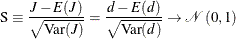
Let  , where
  is the
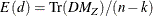
  square matrix of 1s. The mean and variance can be calculated by the formulas
![\begin{equation*} \mr{Var}(d) = 2\{ (n-k)\mr{Tr}\left(DM_{Z}\right)^2-\left[\mr{Tr}\left(DM_{Z}\right)\right]^{2}\} /((n-k)^{2}(n-k+2)) \end{equation*}](images/etsug_panel1021.png)
where  denotes the trace of a particular matrix, Z represents the regressors in the pooled model,
  is the number of observations, k is the number of regressors, and
 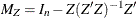 . To calculate
  , let
, let  . Then
![\begin{equation*} \mr{Tr}(DM_{Z})=NT-\mr{Tr}\left(J_{T}\sum _{i=1}^{N}\left[Z_{i}\left(\sum _{j=1}^{N}Z_{j}’Z_{j}\right)^{-1}Z_{i}’\right]\right) \end{equation*}](images/etsug_panel1026.png)
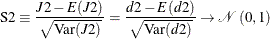
To test for  (no time effects), define
 ![$d2=\left(\sum _{t = 1}^{T}\left[\sum _{i=1}^{N}\hat{u}_{it}\right]^{2}\right)/\left(\sum _{t= 1}^{T}\sum _{i=1}^{N}\hat{u}_{it}^{2}\right)$](images/etsug_panel1028.png) . Then the test statistic is modified as
. Then the test statistic is modified as
![\begin{equation*} J2\equiv \sqrt {\frac{NT}{2(N-1)}}\left[d2-1\right]\xrightarrow {H_{0}^{2}}\mathcal{N}\left(0,1\right) \end{equation*}](images/etsug_panel1029.png)
 can be standardized by
  , and other parameters are unchanged. Therefore,
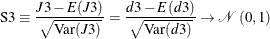
To test for 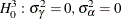 (no cross-sectional and time effects), the test statistic is
 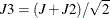 and
and  . To standardize, define
  ,
,
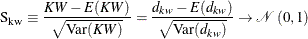
King and Wu (1997) LMMP Test and the SLM Test
King and Wu (1997) derive the locally mean most powerful (LMMP) one-sided test for  and
and  , which coincides with the Honda (1985) UMP test. Baltagi, Chang, and Li (1992) extend the King and Wu (1997) test for
  as follows:
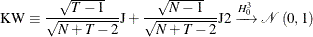
For the standardization, use 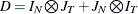 . Define
  ; then
Gourieroux, Holly, and Monfort (1982) LM Test
If one or both variance components ( and
and  ) are small and close to 0, the test statistics J and can be negative. Baltagi, Chang, and Li (1992) follow Gourieroux, Holly, and Monfort (1982) and propose a one-sided LM test for , which is immune to the possible negative values of J and . The test statistic is
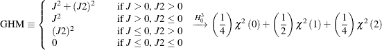
where  is the unit mass at the origin.