The PANEL Procedure
- Overview
- Getting Started
-
Syntax

-
DetailsSpecifying the Input DataSpecifying the Regression ModelUnbalanced DataMissing ValuesComputational ResourcesRestricted EstimatesNotationOne-Way Fixed-Effects ModelTwo-Way Fixed-Effects ModelBalanced PanelsUnbalanced PanelsFirst-Differenced Methods for One-Way and Two-Way ModelsBetween EstimatorsPooled EstimatorOne-Way Random-Effects ModelTwo-Way Random-Effects ModelHausman-Taylor EstimationAmemiya-MaCurdy EstimationParks Method (Autoregressive Model)Da Silva Method (Variance-Component Moving Average Model)Dynamic Panel EstimatorsLinear Hypothesis TestingHeteroscedasticity-Corrected Covariance MatricesHeteroscedasticity- and Autocorrelation-Consistent Covariance MatricesR-SquareSpecification TestsPanel Data Poolability TestPanel Data Cross-Sectional Dependence TestPanel Data Unit Root TestsLagrange Multiplier (LM) Tests for Cross-Sectional and Time EffectsTests for Serial Correlation and Cross-Sectional EffectsTroubleshootingCreating ODS GraphicsOUTPUT OUT= Data SetOUTEST= Data SetOUTTRANS= Data SetPrinted OutputODS Table Names
-
Examples
- References
Hausman-Taylor Estimation
The Hausman and Taylor (1981) model is a hybrid that combines the consistency of a fixed-effects model with the efficiency and applicability of a random-effects model. One-way random-effects models assume exogeneity of the regressors, namely that they be independent of both the cross-sectional and observation-level errors. In cases where some regressors are correlated with the cross-sectional errors, the random effects model can be adjusted to deal with the endogeneity.
Consider the one-way model:
![\[ y_{it}= \Strong{X}_{1it} \bbeta _1 + \Strong{X}_{2it} \bbeta _2 + \Strong{Z}_{1i} \bgamma _1 + \Strong{Z}_{2i} \bgamma _2 + \nu _ i + \epsilon _{it} \hspace{0.2 in} \]](images/etsug_panel0297.png)
The regressors are subdivided so that the  variables vary within cross sections whereas the
  variables do not and would otherwise be dropped from a fixed-effects model. The subscript 1 denotes variables that are independent
of both error terms (exogenous variables), and the subscript 2 denotes variables that are independent of the observation-level
errors
variables do not and would otherwise be dropped from a fixed-effects model. The subscript 1 denotes variables that are independent
of both error terms (exogenous variables), and the subscript 2 denotes variables that are independent of the observation-level
errors  but correlated with cross-sectional errors
  (endogenous variables). The intercept term (if your model has one) is included as part of
  in what follows.
The Hausman-Taylor estimator is an instrumental variables regression on data that are weighted similarly to data for random-effects estimation. In both cases, the weights are functions of the estimated variance components.
Begin with  and
and  . The mean transformation vector is
  and the deviations from the mean transform is
  , where
  is a square matrix of ones of dimension
  .
.
The observation-level variance is estimated from a standard fixed-effects model fit. For  ,
,  , and
, and  , let
, let
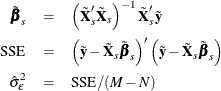
To estimate the cross-sectional error variance, form the mean residuals 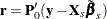 . You can use the mean residuals to obtain intermediate estimates of the coefficients for and
  via two-stage least squares (2SLS) estimation. At the first stage, use
  and as instrumental variables to predict . At the second stage, regress
  on both and the predicted to obtain
  and
and  .
.
To estimate the cross-sectional variance, form 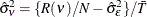 , with
 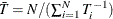 and
and
![\[ R(\nu ) = \left(\Strong{r} - \Strong{Z}_1 \hat\bgamma ^ m_1 - \Strong{Z}_2 \hat\bgamma ^ m_2 \right)’ \left(\Strong{r} - \Strong{Z}_1 \hat\bgamma ^ m_1 - \Strong{Z}_2 \hat\bgamma ^ m_2 \right) \\ \]](images/etsug_panel0317.png)
After variance-component estimation, transform the dependent variable into partial deviations:  . Likewise, transform the regressors to form
  ,
,  ,
,  , and
, and  . The partial weights
  are determined by
  , with
  .
.
Finally, you obtain the Hausman-Taylor estimates by performing 2SLS regression of  on , , , and . For the first-stage regression, use the following instruments:
-
 , the deviations from cross-sectional means for all time-varying variables , for the ith cross section during time period t
-
 , where
  are the means of the time-varying exogenous variables for the ith cross section
-

Multiplication by the factor  is redundant in balanced data, but necessary in the unbalanced case to produce accurate instrumentation; see Gardner (1998).
Let  equal the number of regressors in , and
  equal the number of regressors in . Then the Hausman-Taylor model is identified only if
  ; otherwise, no estimation will take place.
Hausman and Taylor (1981) describe a specification test that compares their model to fixed effects. For a null hypothesis of fixed effects, Hausman’s
m statistic is calculated by comparing the parameter estimates and variance matrices for both models, identically to how it
is calculated for one-way random effects models; for more information, see the section Specification Tests. The degrees of freedom of the test, however, are not based on matrix rank but instead are equal to  .
.