The PANEL Procedure
- Overview
- Getting Started
-
Syntax

-
DetailsSpecifying the Input DataSpecifying the Regression ModelUnbalanced DataMissing ValuesComputational ResourcesRestricted EstimatesNotationOne-Way Fixed-Effects ModelTwo-Way Fixed-Effects ModelBalanced PanelsUnbalanced PanelsFirst-Differenced Methods for One-Way and Two-Way ModelsBetween EstimatorsPooled EstimatorOne-Way Random-Effects ModelTwo-Way Random-Effects ModelHausman-Taylor EstimationAmemiya-MaCurdy EstimationParks Method (Autoregressive Model)Da Silva Method (Variance-Component Moving Average Model)Dynamic Panel EstimatorsLinear Hypothesis TestingHeteroscedasticity-Corrected Covariance MatricesHeteroscedasticity- and Autocorrelation-Consistent Covariance MatricesR-SquareSpecification TestsPanel Data Poolability TestPanel Data Cross-Sectional Dependence TestPanel Data Unit Root TestsLagrange Multiplier (LM) Tests for Cross-Sectional and Time EffectsTests for Serial Correlation and Cross-Sectional EffectsTroubleshootingCreating ODS GraphicsOUTPUT OUT= Data SetOUTEST= Data SetOUTTRANS= Data SetPrinted OutputODS Table Names
-
Examples
- References
Parks Method (Autoregressive Model)
Parks (1967) considered the first-order autoregressive model in which the random errors  ,
,  , and
, and  have the structure
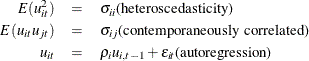
where
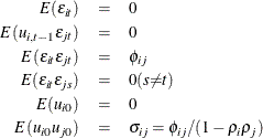
The model assumed is first-order autoregressive with contemporaneous correlation between cross sections. In this model, the covariance matrix for the vector of random errors u can be expressed as
![\begin{eqnarray*} {E}( \Strong{uu} ^{'})=\Strong{V} = \left[\begin{matrix} {\sigma }_{11}P_{11} & {\sigma }_{12}P_{12} & {\ldots } & {\sigma }_{1N}P_{1N} \\ {\sigma }_{21}P_{21} & {\sigma }_{22}P_{22} & {\ldots } & {\sigma }_{2N}P_{2N} \\ {\vdots } & {\vdots } & {\vdots } & {\vdots } \\ {\sigma }_{N1}P_{N1} & {\sigma }_{N2}P_{N2} & {\ldots } & {\sigma }_{NN}P_{NN} \\ \end{matrix} \nonumber \right] \end{eqnarray*}](images/etsug_panel0350.png)
where
![\begin{eqnarray*} P_{ij}= \left[\begin{matrix} 1 & {\rho }_{j} & {\rho }_{j}^{2} & {\ldots } & {\rho }^{T-1}_{j} \\ {\rho }_{i} & 1 & {\rho }_{j} & {\ldots } & {\rho }^{T-2}_{j} \\ {\rho }_{i}^{2} & {\rho }_{i} & 1 & {\ldots } & {\rho }^{T-3}_{j} \\ {\vdots } & {\vdots } & {\vdots } & {\vdots } & {\vdots } \\ {\rho }^{T-1}_{i} & {\rho }^{T-2}_{i} & {\rho }^{T-3}_{i} & {\ldots } & 1 \\ \end{matrix} \nonumber \right] \end{eqnarray*}](images/etsug_panel0351.png)
The matrix V is estimated by a two-stage procedure, and  is then estimated by generalized least squares.
The first step in estimating V involves the use of ordinary least squares to estimate and obtain the fitted residuals, as follows:
is then estimated by generalized least squares.
The first step in estimating V involves the use of ordinary least squares to estimate and obtain the fitted residuals, as follows:
![\[ \hat{\mb{u}} =\mb{y}-\mb{X} \hat{\bbeta }_{OLS} \]](images/etsug_panel0352.png)
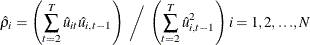
A consistent estimator of the first-order autoregressive parameter is then obtained in the usual manner, as follows:
Finally, the autoregressive characteristic of the data is removed (asymptotically) by the usual transformation of taking
weighted differences. That is, for  ,
,
![\[ y_{i1}\sqrt {1- \hat{\rho }^{2}_{i}}= \sum _{k=1}^{p}{X_{i1k}\mb{{\bbeta }}_{k}} \sqrt {1- \hat{\rho }^{2}_{i}} +u_{i1}\sqrt {1- \hat{\rho }^{2}_{i}} \]](images/etsug_panel0355.png)
![\[ y_{it}- \hat{\rho }_{i} y_{i,t-1} =\sum _{k=1}^{p}{( X_{itk}- \hat{\rho }_{i} \mb{X} _{i,t-1,k}) {\bbeta }_{k}} + u_{it}- \hat{\rho }_{i} u_{i,t-1} t=2,{\ldots },\mi{T} \]](images/etsug_panel0356.png)
which is written
![\[ y^{\ast }_{it}= \sum _{k=1}^{p}{X^{\ast }_{itk} {\bbeta }_{k}}+ u^{\ast }_{it} \; \; i=1, 2, {\ldots }, \mi{N} ; \; \; t=1, 2, {\ldots }, \mi{T} \]](images/etsug_panel0357.png)
Notice that the transformed model has not lost any observations (Seely and Zyskind 1971).
The second step in estimating the covariance matrix V is applying ordinary least squares to the preceding transformed model, obtaining
![\[ \hat{\mb{u}} ^{\ast }= \mb{y} ^{\ast }- \mb{X} ^{\ast } {\bbeta }^{\ast }_{OLS} \]](images/etsug_panel0358.png)
from which the consistent estimator of 
 is calculated as follows:
![\[ s_{ij}=\frac{\hat{\phi }_{ij}}{(1- \hat{\rho }_{i} \hat{\rho }_{j}) } \]](images/etsug_panel0361.png)
where
![\[ \hat{\phi }_{ij}=\frac{1}{(\mi{T} -p)} \sum _{t=1}^{T} \hat{u}^{\ast }_{it} \hat{u}^{\ast }_{jt} \]](images/etsug_panel0362.png)
Estimated generalized least squares (EGLS) then proceeds in the usual manner,
![\[ \hat{\bbeta }_{P}= ({\mb{X} ’}\hat{\mb{V}} ^{-1}\mb{X} )^{-1} {\mb{X} ’}\hat{\mb{V}} ^{-1}\mb{y} \]](images/etsug_panel0363.png)
where  is the derived consistent estimator of V. For computational purposes,
  is obtained directly from the transformed model,
![\[ \hat{\bbeta }_{P}= ({\mb{X} ^{\ast '}}(\hat{\Phi }^{-1}{\otimes }I_{T}) \mb{X} ^{\ast })^{-1}{\mb{X} ^{\ast '}} (\hat{\Phi }^{-1}{\otimes }I_{T}) \mb{y} ^{\ast } \]](images/etsug_panel0366.png)
where ![${\hat{\Phi }= [\hat{\phi }_{ij}]_{i,j=1,{\ldots },N} }$](images/etsug_panel0367.png) .
.
The preceding procedure is equivalent to Zellner’s two-stage methodology applied to the transformed model (Zellner 1962).
Parks demonstrates that this estimator is consistent and asymptotically, normally distributed with
![\[ \mr{Var}(\hat{\bbeta }_{P})= ({\mb{X} ’}\mb{V} ^{-1}\mb{X} )^{-1} \]](images/etsug_panel0368.png)
Standard Corrections
For the PARKS option, the first-order autocorrelation coefficient must be estimated for each cross section. Let  be the
  vector of true parameters and
  be the corresponding vector of estimates. Then, to ensure that only range-preserving estimates are used in PROC PANEL, the
following modification for R is made:
be the corresponding vector of estimates. Then, to ensure that only range-preserving estimates are used in PROC PANEL, the
following modification for R is made:
![\[ r_{i} = \begin{cases} r_{i} & \mr{if} \hspace{.1 in}{|r_{i}|}<1 \\ \mr{max}(.95, \mr{rmax}) & \mr{if}\hspace{.1 in} r_{i}{\ge }1 \\ \mr{min}(-.95, \mr{rmin}) & \mr{if}\hspace{.1 in} r_{i}{\le }-1 \end{cases} \]](images/etsug_panel0372.png)
where
![\[ \mr{rmax} = \begin{cases} 0 & \mr{if}\hspace{.1 in} r_{i} < 0 \hspace{.1 in}\mr{or}\hspace{.1 in} r_{i}{\ge }1\hspace{.1 in} \forall i \\ \mathop {\mr{max}}\limits _{j} [ r_{j} : 0 {\le } r_{j} < 1 ] & \mr{otherwise} \end{cases} \]](images/etsug_panel0373.png)
and
![\[ \mr{rmin }= \begin{cases} 0 & \mr{if} \hspace{.1 in}r_{i} > 0 \hspace{.1 in}\mr{or}\hspace{.1 in} r_{i}{\le }-1\hspace{.1 in} \forall i \\ \mathop {\mr{max}}\limits _{j} [ r_{j} : -1 < r_{j} {\le } 0 ] & \mr{otherwise} \end{cases} \]](images/etsug_panel0374.png)
Whenever this correction is made, a warning message is printed.