The PANEL Procedure
- Overview
- Getting Started
-
Syntax

-
DetailsSpecifying the Input DataSpecifying the Regression ModelUnbalanced DataMissing ValuesComputational ResourcesRestricted EstimatesNotationOne-Way Fixed-Effects ModelTwo-Way Fixed-Effects ModelBalanced PanelsUnbalanced PanelsFirst-Differenced Methods for One-Way and Two-Way ModelsBetween EstimatorsPooled EstimatorOne-Way Random-Effects ModelTwo-Way Random-Effects ModelHausman-Taylor EstimationAmemiya-MaCurdy EstimationParks Method (Autoregressive Model)Da Silva Method (Variance-Component Moving Average Model)Dynamic Panel EstimatorsLinear Hypothesis TestingHeteroscedasticity-Corrected Covariance MatricesHeteroscedasticity- and Autocorrelation-Consistent Covariance MatricesR-SquareSpecification TestsPanel Data Poolability TestPanel Data Cross-Sectional Dependence TestPanel Data Unit Root TestsLagrange Multiplier (LM) Tests for Cross-Sectional and Time EffectsTests for Serial Correlation and Cross-Sectional EffectsTroubleshootingCreating ODS GraphicsOUTPUT OUT= Data SetOUTEST= Data SetOUTTRANS= Data SetPrinted OutputODS Table Names
-
Examples
- References
Da Silva Method (Variance-Component Moving Average Model)
The Da Silva method assumes that the observed value of the dependent variable at the tth time point on the ith cross-sectional unit can be expressed as
![\[ y_{it}= \mb{x} _{it}^{'}{\beta } + a_{i}+ b_{t}+ e_{it} \hspace{.3 in} i=1, {\ldots }, \mi{N} ;t=1, {\ldots }, \mi{T} \]](images/etsug_panel0375.png)
where
-
 is a vector of explanatory variables for the tth time point and ith cross-sectional unit
-
 is the vector of parameters
-
 is a time-invariant, cross-sectional unit effect
-
 is a cross-sectionally invariant time effect
-
 is a residual effect unaccounted for by the explanatory variables and the specific time and cross-sectional unit effects
Since the observations are arranged first by cross sections, then by time periods within cross sections, these equations can be written in matrix notation as
![\[ \mb{y} =\mb{X} {\beta }+\mb{u} \]](images/etsug_panel0381.png)
where
![\[ \mb{u} =(\mb{a} {\otimes }\mb{1} _{T})+(\mb{1} _{N}{\otimes }\mb{b} )+\mb{e} \]](images/etsug_panel0382.png)
![\[ \mb{y} = (y_{11},{\ldots },y_{1T}, y_{21},{\ldots },y_{NT}{)’} \]](images/etsug_panel0383.png)
![\[ \mb{X} =(\mb{x} _{11},{\ldots },\mb{x} _{1T},\mb{x} _{21},{\ldots } ,\mb{x} _{NT}{)’} \]](images/etsug_panel0384.png)
![\[ \mb{a} =(a_{1}{\ldots }a_{N}{)’} \]](images/etsug_panel0385.png)
![\[ \mb{b} =(b_{1}{\ldots }b_{T}{)’} \]](images/etsug_panel0386.png)
![\[ \mb{e} = (e_{11},{\ldots },e_{1T}, e_{21},{\ldots },e_{NT}{)’} \]](images/etsug_panel0387.png)
Here 1  is an
is an  vector with all elements equal to 1, and
  denotes the Kronecker product.
The following conditions are assumed:
-
 is a sequence of nonstochastic, known
  vectors in
  whose elements are uniformly bounded in . The matrix X has a full column rank p.
-
 is a
is a  constant vector of unknown parameters.
-
a is a vector of uncorrelated random variables such that
 and
and  ,
,  .
.
-
b is a vector of uncorrelated random variables such that
 and
and  where
where  and
and  .
.
-
 is a sample of a realization of a finite moving-average time series of order
  for each i ; hence,
![\[ e_{it}={\alpha }_{0} {\epsilon }_{it}+ {\alpha }_{1} {\epsilon }_{it-1}+{\ldots }+ {\alpha }_{m} {\epsilon }_{it-m} \; \; \; \; t=1,{\ldots },\mi{T} ; i=1,{\ldots },\mi{N} \]](images/etsug_panel0403.png)
where
 are unknown constants such that
  and
and  , and
, and  is a white noise process for each i—that is, a sequence of uncorrelated random variables with
 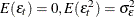 , and
, and  . for
. for  are mutually uncorrelated.
-
The sets of random variables
 ,
,  , and
, and  for are mutually uncorrelated.
-
The random terms have normal distributions
 and
and  for
for  and
and  .
.
If assumptions 1–6 are satisfied, then
![\[ {E}(\mb{y} )=\mb{X} {\beta } \]](images/etsug_panel0418.png)
and
![\[ \mr{var}(\mb{y} )= {\sigma }^{2}_{a} (I_{N}{\otimes }J_{T})+ {\sigma }^{2}_{b}(J_{N}{\otimes }I_{T})+ (I_{N}{\otimes }{\Psi }_{T}) \]](images/etsug_panel0419.png)
where  is a
is a  matrix with elements
  as follows:
![\[ \mr{Cov}( e_{it} e_{is})= \begin{cases} {\psi }({|t-s|}) & \mr{if}\hspace{.1 in} {|t-s|} {\le } m \\ 0 & \mr{if} \hspace{.1 in}{|t-s|} > m \end{cases} \]](images/etsug_panel0423.png)
where 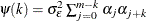 for
for  . For the definition of
  ,
,  ,
,  , and
, and  , see the section Fuller and Battese Method.
The covariance matrix, denoted by V, can be written in the form
![\[ \mb{V} = {\sigma }^{2}_{a}(I_{N}{\otimes }J_{T}) + {\sigma }^{2}_{b}(J_{N}{\otimes }I_{T}) +\sum _{k=0}^{m}{{\psi }(k)(I_{N}{\otimes } {\Psi }^{(k)}_{T})} \]](images/etsug_panel0430.png)
where  , and, for k =1,
 , m,
, m,  is a band matrix whose kth off-diagonal elements are 1’s and all other elements are 0’s.
Thus, the covariance matrix of the vector of observations y has the form
![\[ {\mr{Var}}(\mb{y} )=\sum _{k=1}^{m+3}{{\nu }_{k}V_{k}} \]](images/etsug_panel0434.png)
where
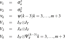
The estimator of is a two-step GLS-type estimator—that is, GLS with the unknown covariance matrix replaced by a suitable estimator of V. It is obtained by substituting Seely estimates for the scalar multiples 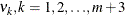 .
.
Seely (1969) presents a general theory of unbiased estimation when the choice of estimators is restricted to finite dimensional vector
spaces, with a special emphasis on quadratic estimation of functions of the form  .
.
The parameters  (i =1,, n) are associated with a linear model E(y )=X
  with covariance matrix
  where
where  (i =1, , n) are real symmetric matrices. The method is also discussed by Seely (1970b, 1970a); Seely and Zyskind (1971). Seely and Soong (1971) consider the MINQUE principle, using an approach along the lines of Seely (1969).