The LOGISTIC Procedure
- Overview
- Getting Started
-
Syntax
 PROC LOGISTIC StatementBY StatementCLASS StatementCODE StatementCONTRAST StatementEFFECT StatementEFFECTPLOT StatementESTIMATE StatementEXACT StatementEXACTOPTIONS StatementFREQ StatementID StatementLSMEANS StatementLSMESTIMATE StatementMODEL StatementNLOPTIONS StatementODDSRATIO StatementOUTPUT StatementROC StatementROCCONTRAST StatementSCORE StatementSLICE StatementSTORE StatementSTRATA StatementTEST StatementUNITS StatementWEIGHT Statement
 -
DetailsMissing ValuesResponse Level OrderingLink Functions and the Corresponding DistributionsDetermining Observations for Likelihood ContributionsIterative Algorithms for Model FittingConvergence CriteriaExistence of Maximum Likelihood EstimatesEffect-Selection MethodsModel Fitting InformationGeneralized Coefficient of DeterminationScore Statistics and TestsConfidence Intervals for ParametersOdds Ratio EstimationRank Correlation of Observed Responses and Predicted ProbabilitiesLinear Predictor, Predicted Probability, and Confidence LimitsClassification TableOverdispersionThe Hosmer-Lemeshow Goodness-of-Fit TestReceiver Operating Characteristic CurvesTesting Linear Hypotheses about the Regression CoefficientsJoint Tests and Type 3 TestsRegression DiagnosticsScoring Data SetsConditional Logistic RegressionExact Conditional Logistic RegressionInput and Output Data SetsComputational ResourcesDisplayed OutputODS Table NamesODS Graphics
-
ExamplesStepwise Logistic Regression and Predicted ValuesLogistic Modeling with Categorical PredictorsOrdinal Logistic RegressionNominal Response Data: Generalized Logits ModelStratified SamplingLogistic Regression DiagnosticsROC Curve, Customized Odds Ratios, Goodness-of-Fit Statistics, R-Square, and Confidence LimitsComparing Receiver Operating Characteristic CurvesGoodness-of-Fit Tests and SubpopulationsOverdispersionConditional Logistic Regression for Matched Pairs DataExact Conditional Logistic RegressionFirth’s Penalized Likelihood Compared with Other ApproachesComplementary Log-Log Model for Infection RatesComplementary Log-Log Model for Interval-Censored Survival TimesScoring Data SetsUsing the LSMEANS StatementPartial Proportional Odds Model
- References
EXACTOPTIONS Statement
-
EXACTOPTIONS options;
The EXACTOPTIONS statement specifies options that apply to every EXACT statement in the program. The following options are available:
- ABSFCONV=value
-
specifies the absolute function convergence criterion. Convergence requires a small change in the log-likelihood function in subsequent iterations,
![\[ |l_ i - l_{i-1}| < \mi{value} \]](images/statug_logistic0076.png)
where
 is the value of the log-likelihood function at iteration i.
By default, ABSFCONV=1E–12. You can also specify the FCONV= and XCONV= criteria; optimizations are terminated as soon as one criterion is satisfied.
- ADDTOBS
-
adds the observed sufficient statistic to the sampled exact distribution if the statistic was not sampled. This option has no effect unless the METHOD=NETWORKMC or METHOD=MCMC option is specified and the ESTIMATE option is specified in the EXACT statement. If the observed statistic has not been sampled, then the parameter estimate does not exist; by specifying this option, you can produce (biased) estimates.
- BUILDSUBSETS
-
builds every distribution for sampling. By default, some exact distributions are created by taking a subset of a previously generated exact distribution. When the METHOD=NETWORKMC or METHOD=MCMC option is invoked, this subsetting behavior has the effect of using fewer than the desired n samples; see the N= option for more details. Use the BUILDSUBSETS option to suppress this subsetting.
- EPSILON=value
-
controls how the partial sums
 are compared. value must be between 0 and 1; by default, value=1E–8.
- FCONV=value
-
specifies the relative function convergence criterion. Convergence requires a small relative change in the log-likelihood function in subsequent iterations,
![\[ \frac{ |l_ i - l_{i-1}|}{|l_{i-1}| + {\mbox{1E--6}}} < \mi{value} \]](images/statug_logistic0079.png)
where
is the value of the log likelihood at iteration i.
By default, FCONV=1E–8. You can also specify the ABSFCONV= and XCONV= criteria; if you specify more than one criterion, then optimizations are terminated as soon as one criterion is satisfied.
-
MAXSWAP=n
MAXR=n -
specifies the maximum number of swaps for each sample that PROC LOGISTIC makes when you specify the METHOD=MCMC option. If an intercept or a stratum is conditioned out, then n swaps are performed: one event is changed to a nonevent, and one nonevent is changed to an event. Although you might need large values of n in order to transition between any two points in the exact distribution, such values quickly increase computation time. By default, MAXSWAP=2.
- MAXTIME=seconds
-
specifies the maximum clock time (in seconds) that PROC LOGISTIC can use to calculate the exact distributions. If the limit is exceeded, the procedure halts all computations and prints a note to the SAS log. The default maximum clock time is seven days.
- METHOD=keyword
-
specifies which exact conditional algorithm to use for every EXACT statement specified. You can specify one of the following keywords:
- DIRECT
-
invokes the multivariate shift algorithm of Hirji, Mehta, and Patel (1987). This method directly builds the exact distribution, but it can require an excessive amount of memory in its intermediate stages. METHOD=DIRECT is invoked by default when you are conditioning out at most the intercept, or when the LINK=GLOGIT option is specified in the MODEL statement.
- NETWORK
-
invokes an algorithm described in Mehta, Patel, and Senchaudhuri (1992). This method builds a network for each parameter that you are conditioning out, combines the networks, then uses the multivariate shift algorithm to create the exact distribution. The NETWORK method can be faster and require less memory than the DIRECT method. The NETWORK method is invoked by default for most analyses.
- NETWORKMC
-
invokes the hybrid network and Monte Carlo algorithm of Mehta, Patel, and Senchaudhuri (1992). This method creates a network, then samples from that network; this method does not reject any of the samples at the cost of using a large amount of memory to create the network. METHOD=NETWORKMC is most useful for producing parameter estimates for problems that are too large for the DIRECT and NETWORK methods to handle and for which asymptotic methods are invalid—for example, for sparse data on a large grid.
- MCMC
-
invokes the Markov chain Monte Carlo (MCMC) algorithm of Forster, McDonald, and Smith (2003). This method uses a Metropolis-Hastings algorithm to generate samples from the exact distribution by repeatedly perturbing the response vector to obtain a new response vector while maintaining the sufficient statistics for the nuisance parameters. You must also condition out the intercept or the strata. (Using notation from Zamar et al. 2007, the current implementation samples from
 , does not explicitly sample for v = 0, allows candidates v and –v, allows d < 0, and limits r by the number of observations.) The sampling is divided into parallel threads, where the number of threads is the value of
the SAS system option CPUCOUNT=. The MCMC method is most useful for problems for which the NETWORKMC method has difficulty
generating the network and for which asymptotic results are suspect; however, to make sure you are sampling from the equilibrium
distribution, you should run your program multiple times and increase the N=
and MAXSWAP=
values until you believe that your results are stable. The MCMC method can take a large amount of time, depending on the
number of observations in your data set, the number of samples, and the number of swaps.
, does not explicitly sample for v = 0, allows candidates v and –v, allows d < 0, and limits r by the number of observations.) The sampling is divided into parallel threads, where the number of threads is the value of
the SAS system option CPUCOUNT=. The MCMC method is most useful for problems for which the NETWORKMC method has difficulty
generating the network and for which asymptotic results are suspect; however, to make sure you are sampling from the equilibrium
distribution, you should run your program multiple times and increase the N=
and MAXSWAP=
values until you believe that your results are stable. The MCMC method can take a large amount of time, depending on the
number of observations in your data set, the number of samples, and the number of swaps.
- N=n
-
specifies the number of Monte Carlo samples to take when you specify the METHOD=NETWORKMC or METHOD=MCMC option. By default, n = 10,000. If PROC LOGISTIC cannot obtain n samples because of a lack of memory, then a note is printed in the SAS log (the number of valid samples is also reported in the listing) and the analysis continues.
The number of samples used to produce any particular statistic might be smaller than n. For example, let X1 and X2 be continuous variables, denote their joint distribution by f(X1,X2), and let f(X1 | X2 = x2) denote the marginal distribution of X1 conditioned on the observed value of X2. If you request the JOINT test of X1 and X2, then n samples are used to generate the estimate
 (X1,X2) of f(X1,X2), from which the test is computed. However, the parameter estimate for X1 is computed from the subset of (X1,X2) that has X2 = x2, and this subset need not contain n samples. Similarly, the distribution for each level of a classification variable is created by extracting the appropriate
subset from the joint distribution for the CLASS
variable.
(X1,X2) of f(X1,X2), from which the test is computed. However, the parameter estimate for X1 is computed from the subset of (X1,X2) that has X2 = x2, and this subset need not contain n samples. Similarly, the distribution for each level of a classification variable is created by extracting the appropriate
subset from the joint distribution for the CLASS
variable.
In some cases, the marginal sample size can be too small to admit accurate estimation of a particular statistic; a note is printed in the SAS log when a marginal sample size is less than 100. Increasing n increases the number of samples used in a marginal distribution; however, if you want to control the sample size exactly, you can either specify the BUILDSUBSETS option or do both of the following:
-
NBI=n
BURNIN=n -
specifies the number of burn-in samples that are discarded when you specify the METHOD=MCMC option. By default, NBI=0.
- NOLOGSCALE
-
specifies that computations for the exact conditional models be computed by using normal scaling. Log scaling can handle numerically larger problems than normal scaling; however, computations in the log scale are slower than computations in normal scale.
- NTHIN=n
-
controls the thinning rate of the sampling when you specify the METHOD=MCMC option. Every nth sample is kept and the rest are discarded. By default, NTHIN=1.
- ONDISK
-
uses disk space instead of random access memory to build the exact conditional distribution. Use this option to handle larger problems at the cost of slower processing.
- SEED=seed
-
specifies the initial seed for the random number generator used to take the Monte Carlo samples when you specify the METHOD=NETWORKMC or METHOD=MCMC option. The value of the SEED= option must be an integer. If you do not specify a seed, or if you specify a value less than or equal to 0, then PROC LOGISTIC uses the time of day from the computer’s clock to generate an initial seed.
- STATUSN=number
-
prints a status line in the SAS log after every number of Monte Carlo samples when you specify the METHOD=NETWORKMC or METHOD=MCMC option. When you specify METHOD=MCMC , the actual number that is used depends on the number of threads used in the computations. The number of samples that are taken and the current exact p-value for testing the significance of the model are displayed. You can use this status line to track the progress of the computation of the exact conditional distributions.
- STATUSTIME=seconds
-
specifies the time interval (in seconds) for printing a status line in the SAS log. You can use this status line to track the progress of the computation of the exact conditional distributions. The time interval that you specify is approximate; the actual time interval varies. By default, no status reports are produced.
- XCONV=value
-
specifies the relative parameter convergence criterion. Convergence requires a small relative parameter change in subsequent iterations,
![\[ \max _ j |\delta _ j^{(i)}| < \mi{value} \]](images/statug_logistic0082.png)
where
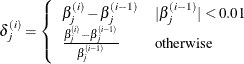
and
 is the estimate of the jth parameter at iteration i.
By default, XCONV=1E–4. You can also specify the ABSFCONV= and FCONV= criteria; if more than one criterion is specified, then optimizations are terminated as soon as one criterion is satisfied.