The LOGISTIC Procedure
- Overview
- Getting Started
-
Syntax
 PROC LOGISTIC StatementBY StatementCLASS StatementCODE StatementCONTRAST StatementEFFECT StatementEFFECTPLOT StatementESTIMATE StatementEXACT StatementEXACTOPTIONS StatementFREQ StatementID StatementLSMEANS StatementLSMESTIMATE StatementMODEL StatementNLOPTIONS StatementODDSRATIO StatementOUTPUT StatementROC StatementROCCONTRAST StatementSCORE StatementSLICE StatementSTORE StatementSTRATA StatementTEST StatementUNITS StatementWEIGHT Statement
 -
DetailsMissing ValuesResponse Level OrderingLink Functions and the Corresponding DistributionsDetermining Observations for Likelihood ContributionsIterative Algorithms for Model FittingConvergence CriteriaExistence of Maximum Likelihood EstimatesEffect-Selection MethodsModel Fitting InformationGeneralized Coefficient of DeterminationScore Statistics and TestsConfidence Intervals for ParametersOdds Ratio EstimationRank Correlation of Observed Responses and Predicted ProbabilitiesLinear Predictor, Predicted Probability, and Confidence LimitsClassification TableOverdispersionThe Hosmer-Lemeshow Goodness-of-Fit TestReceiver Operating Characteristic CurvesTesting Linear Hypotheses about the Regression CoefficientsJoint Tests and Type 3 TestsRegression DiagnosticsScoring Data SetsConditional Logistic RegressionExact Conditional Logistic RegressionInput and Output Data SetsComputational ResourcesDisplayed OutputODS Table NamesODS Graphics
-
ExamplesStepwise Logistic Regression and Predicted ValuesLogistic Modeling with Categorical PredictorsOrdinal Logistic RegressionNominal Response Data: Generalized Logits ModelStratified SamplingLogistic Regression DiagnosticsROC Curve, Customized Odds Ratios, Goodness-of-Fit Statistics, R-Square, and Confidence LimitsComparing Receiver Operating Characteristic CurvesGoodness-of-Fit Tests and SubpopulationsOverdispersionConditional Logistic Regression for Matched Pairs DataExact Conditional Logistic RegressionFirth’s Penalized Likelihood Compared with Other ApproachesComplementary Log-Log Model for Infection RatesComplementary Log-Log Model for Interval-Censored Survival TimesScoring Data SetsUsing the LSMEANS StatementPartial Proportional Odds Model
- References
Example 72.3 Ordinal Logistic Regression
Consider a study of the effects on taste of various cheese additives. Researchers tested four cheese additives and obtained
52 response ratings for each additive. Each response was measured on a scale of nine categories ranging from strong dislike
(1) to excellent taste (9). The data, given in McCullagh and Nelder (1989, p. 175) in the form of a two-way frequency table of additive by rating, are saved in the data set Cheese by using the following program. The variable y contains the response rating. The variable Additive specifies the cheese additive (1, 2, 3, or 4). The variable freq gives the frequency with which each additive received each rating.
data Cheese;
   do Additive = 1 to 4;
      do y = 1 to 9;
         input freq @@;
         output;
      end;
   end;
   label y='Taste Rating';
   datalines;
0  0  1  7  8  8 19  8  1
6  9 12 11  7  6  1  0  0
1  1  6  8 23  7  5  1  0
0  0  0  1  3  7 14 16 11
;
The response variable y is ordinally scaled. A cumulative logit model is used to investigate the effects of the cheese additives on taste. The following
statements invoke PROC LOGISTIC to fit this model with y as the response variable and three indicator variables as explanatory variables, with the fourth additive as the reference
level. With this parameterization, each Additive parameter compares an additive to the fourth additive. The COVB
option displays the estimated covariance matrix, and the NOODDSRATIO
option suppresses the default odds ratio table. The ODDSRATIO
statement computes odds ratios for all combinations of the Additive levels. The PLOTS
option produces a graphical display of the odds ratios, and the EFFECTPLOT
statement displays the predicted probabilities.
ods graphics on;
proc logistic data=Cheese plots(only)=oddsratio(range=clip);
   freq freq;
   class Additive (param=ref ref='4');
   model y=Additive / covb nooddsratio;
   oddsratio Additive;
   effectplot / polybar;
   title 'Multiple Response Cheese Tasting Experiment';
run;
The "Response Profile" table in Output 72.3.1 shows that the strong dislike (y=1) end of the rating scale is associated with lower Ordered Values in the "Response Profile" table; hence the probability
of disliking the additives is modeled.
The score chi-square for testing the proportional odds assumption is 17.287, which is not significant with respect to a chi-square
distribution with 21 degrees of freedom  . This indicates that the proportional odds assumption is reasonable. The positive value (1.6128) for the parameter estimate
for
. This indicates that the proportional odds assumption is reasonable. The positive value (1.6128) for the parameter estimate
for Additive1 indicates a tendency toward the lower-numbered categories of the first cheese additive relative to the fourth. In other words,
the fourth additive tastes better than the first additive. The second and third additives are both less favorable than the
fourth additive. The relative magnitudes of these slope estimates imply the preference ordering: fourth, first, third, second.
Output 72.3.1: Proportional Odds Model Regression Analysis
| Analysis of Maximum Likelihood Estimates | ||||||
|---|---|---|---|---|---|---|
| Parameter | DF | Estimate | Standard Error |
Wald Chi-Square |
Pr > ChiSq | |
| Intercept | 1 | 1 | -7.0801 | 0.5624 | 158.4851 | <.0001 |
| Intercept | 2 | 1 | -6.0249 | 0.4755 | 160.5500 | <.0001 |
| Intercept | 3 | 1 | -4.9254 | 0.4272 | 132.9484 | <.0001 |
| Intercept | 4 | 1 | -3.8568 | 0.3902 | 97.7087 | <.0001 |
| Intercept | 5 | 1 | -2.5205 | 0.3431 | 53.9704 | <.0001 |
| Intercept | 6 | 1 | -1.5685 | 0.3086 | 25.8374 | <.0001 |
| Intercept | 7 | 1 | -0.0669 | 0.2658 | 0.0633 | 0.8013 |
| Intercept | 8 | 1 | 1.4930 | 0.3310 | 20.3439 | <.0001 |
| Additive | 1 | 1 | 1.6128 | 0.3778 | 18.2265 | <.0001 |
| Additive | 2 | 1 | 4.9645 | 0.4741 | 109.6427 | <.0001 |
| Additive | 3 | 1 | 3.3227 | 0.4251 | 61.0931 | <.0001 |
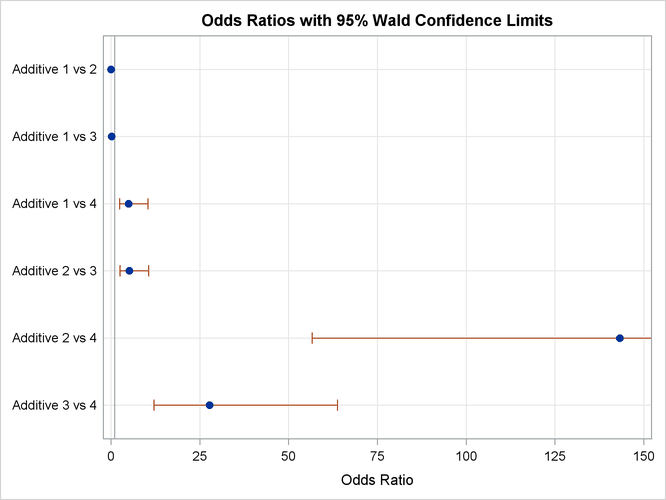
The odds ratio results in Output 72.3.2 show the preferences more clearly. For example, the "Additive 1 vs 4" odds ratio says that the first additive has 5.017 times the odds of receiving a lower score than the fourth additive; that is, the first additive is 5.017 times more likely than the fourth additive to receive a lower score. Output 72.3.3 displays the odds ratios graphically; the range of the confidence limits is truncated by the RANGE=CLIP option, so you can see that "1" is not contained in any of the intervals.
Output 72.3.2: Odds Ratios of All Pairs of Additive Levels
| Odds Ratio Estimates and Wald Confidence Intervals | |||
|---|---|---|---|
| Odds Ratio | Estimate | 95% Confidence Limits | |
| Additive 1 vs 2 | 0.035 | 0.015 | 0.080 |
| Additive 1 vs 3 | 0.181 | 0.087 | 0.376 |
| Additive 1 vs 4 | 5.017 | 2.393 | 10.520 |
| Additive 2 vs 3 | 5.165 | 2.482 | 10.746 |
| Additive 2 vs 4 | 143.241 | 56.558 | 362.777 |
| Additive 3 vs 4 | 27.734 | 12.055 | 63.805 |
Output 72.3.3: Plot of Odds Ratios for Additive
The estimated covariance matrix of the parameters is displayed in Output 72.3.4.
Output 72.3.4: Estimated Covariance Matrix
| Estimated Covariance Matrix | |||||||||||
|---|---|---|---|---|---|---|---|---|---|---|---|
| Parameter | Intercept_1 | Intercept_2 | Intercept_3 | Intercept_4 | Intercept_5 | Intercept_6 | Intercept_7 | Intercept_8 | Additive1 | Additive2 | Additive3 |
| Intercept_1 | 0.316291 | 0.219581 | 0.176278 | 0.147694 | 0.114024 | 0.091085 | 0.057814 | 0.041304 | -0.09419 | -0.18686 | -0.13565 |
| Intercept_2 | 0.219581 | 0.226095 | 0.177806 | 0.147933 | 0.11403 | 0.091081 | 0.057813 | 0.041304 | -0.09421 | -0.18161 | -0.13569 |
| Intercept_3 | 0.176278 | 0.177806 | 0.182473 | 0.148844 | 0.114092 | 0.091074 | 0.057807 | 0.0413 | -0.09427 | -0.1687 | -0.1352 |
| Intercept_4 | 0.147694 | 0.147933 | 0.148844 | 0.152235 | 0.114512 | 0.091109 | 0.05778 | 0.041277 | -0.09428 | -0.14717 | -0.13118 |
| Intercept_5 | 0.114024 | 0.11403 | 0.114092 | 0.114512 | 0.117713 | 0.091821 | 0.057721 | 0.041162 | -0.09246 | -0.11415 | -0.11207 |
| Intercept_6 | 0.091085 | 0.091081 | 0.091074 | 0.091109 | 0.091821 | 0.09522 | 0.058312 | 0.041324 | -0.08521 | -0.09113 | -0.09122 |
| Intercept_7 | 0.057814 | 0.057813 | 0.057807 | 0.05778 | 0.057721 | 0.058312 | 0.07064 | 0.04878 | -0.06041 | -0.05781 | -0.05802 |
| Intercept_8 | 0.041304 | 0.041304 | 0.0413 | 0.041277 | 0.041162 | 0.041324 | 0.04878 | 0.109562 | -0.04436 | -0.0413 | -0.04143 |
| Additive1 | -0.09419 | -0.09421 | -0.09427 | -0.09428 | -0.09246 | -0.08521 | -0.06041 | -0.04436 | 0.142715 | 0.094072 | 0.092128 |
| Additive2 | -0.18686 | -0.18161 | -0.1687 | -0.14717 | -0.11415 | -0.09113 | -0.05781 | -0.0413 | 0.094072 | 0.22479 | 0.132877 |
| Additive3 | -0.13565 | -0.13569 | -0.1352 | -0.13118 | -0.11207 | -0.09122 | -0.05802 | -0.04143 | 0.092128 | 0.132877 | 0.180709 |
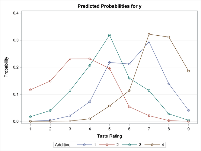
Output 72.3.5 displays the probability of each taste rating y within each additive. You can see that Additive=1 mostly receives ratings of 5 to 7, Additive=2 mostly receives ratings of 2 to 5, Additive=3 mostly receives ratings of 4 to 6, and Additive=4 mostly receives ratings of 7 to 9, which also confirms the previously discussed preference orderings.
Output 72.3.5: Model-Predicted Probabilities
Alternatively, you can use an adjacent-category logit model. The following statements invoke PROC LOGISTIC to fit this model:
proc logistic data=Cheese
   plots(only)=effect(x=y sliceby=additive connect yrange=(0,0.4));
   freq freq;
   class Additive (param=ref ref='4');
   model y=Additive / nooddsratio link=alogit;
   oddsratio Additive;
   title 'Multiple Response Cheese Tasting Experiment';
run;
You can see that the parameter estimates for the intercepts in Output 72.3.6 are no longer strictly increasing, as they are for the cumulative model in Output 72.3.1.
Output 72.3.6: Adjacent-Category Logistic Regression Analysis
| Multiple Response Cheese Tasting Experiment |
| Analysis of Maximum Likelihood Estimates | ||||||
|---|---|---|---|---|---|---|
| Parameter | DF | Estimate | Standard Error |
Wald Chi-Square |
Pr > ChiSq | |
| Intercept | 1 | 1 | -2.2262 | 0.5542 | 16.1350 | <.0001 |
| Intercept | 2 | 1 | -2.4238 | 0.4620 | 27.5216 | <.0001 |
| Intercept | 3 | 1 | -1.9852 | 0.3800 | 27.2909 | <.0001 |
| Intercept | 4 | 1 | -1.8164 | 0.3294 | 30.4096 | <.0001 |
| Intercept | 5 | 1 | -0.6908 | 0.3097 | 4.9737 | 0.0257 |
| Intercept | 6 | 1 | -1.0433 | 0.2841 | 13.4902 | 0.0002 |
| Intercept | 7 | 1 | 0.0322 | 0.2667 | 0.0146 | 0.9040 |
| Intercept | 8 | 1 | 0.5160 | 0.3527 | 2.1402 | 0.1435 |
| Additive | 1 | 1 | 0.7172 | 0.1783 | 16.1776 | <.0001 |
| Additive | 2 | 1 | 1.9838 | 0.2463 | 64.8748 | <.0001 |
| Additive | 3 | 1 | 1.3826 | 0.2122 | 42.4478 | <.0001 |
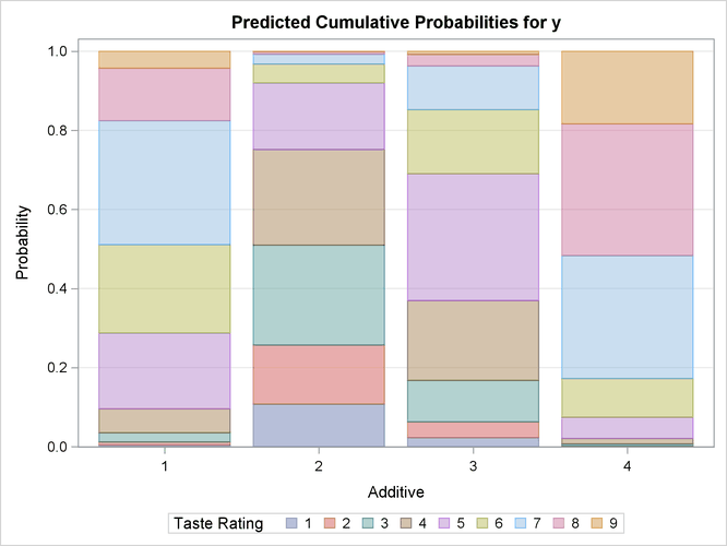
The odds ratio results in Output 72.3.7 show the same preferences that you obtain from the proportional odds model. Output 72.3.8 displays the probability of each additive according to the taste rating.
Output 72.3.7: Odds Ratios of All Pairs of Additive Levels
Output 72.3.8: Model-Predicted Probabilities