The LOGISTIC Procedure
- Overview
- Getting Started
-
Syntax
 PROC LOGISTIC StatementBY StatementCLASS StatementCODE StatementCONTRAST StatementEFFECT StatementEFFECTPLOT StatementESTIMATE StatementEXACT StatementEXACTOPTIONS StatementFREQ StatementID StatementLSMEANS StatementLSMESTIMATE StatementMODEL StatementNLOPTIONS StatementODDSRATIO StatementOUTPUT StatementROC StatementROCCONTRAST StatementSCORE StatementSLICE StatementSTORE StatementSTRATA StatementTEST StatementUNITS StatementWEIGHT Statement
 -
DetailsMissing ValuesResponse Level OrderingLink Functions and the Corresponding DistributionsDetermining Observations for Likelihood ContributionsIterative Algorithms for Model FittingConvergence CriteriaExistence of Maximum Likelihood EstimatesEffect-Selection MethodsModel Fitting InformationGeneralized Coefficient of DeterminationScore Statistics and TestsConfidence Intervals for ParametersOdds Ratio EstimationRank Correlation of Observed Responses and Predicted ProbabilitiesLinear Predictor, Predicted Probability, and Confidence LimitsClassification TableOverdispersionThe Hosmer-Lemeshow Goodness-of-Fit TestReceiver Operating Characteristic CurvesTesting Linear Hypotheses about the Regression CoefficientsJoint Tests and Type 3 TestsRegression DiagnosticsScoring Data SetsConditional Logistic RegressionExact Conditional Logistic RegressionInput and Output Data SetsComputational ResourcesDisplayed OutputODS Table NamesODS Graphics
-
ExamplesStepwise Logistic Regression and Predicted ValuesLogistic Modeling with Categorical PredictorsOrdinal Logistic RegressionNominal Response Data: Generalized Logits ModelStratified SamplingLogistic Regression DiagnosticsROC Curve, Customized Odds Ratios, Goodness-of-Fit Statistics, R-Square, and Confidence LimitsComparing Receiver Operating Characteristic CurvesGoodness-of-Fit Tests and SubpopulationsOverdispersionConditional Logistic Regression for Matched Pairs DataExact Conditional Logistic RegressionFirth’s Penalized Likelihood Compared with Other ApproachesComplementary Log-Log Model for Infection RatesComplementary Log-Log Model for Interval-Censored Survival TimesScoring Data SetsUsing the LSMEANS StatementPartial Proportional Odds Model
- References
Example 72.6 Logistic Regression Diagnostics
In a controlled experiment to study the effect of the rate and volume of air intake on a transient reflex vasoconstriction in the skin of the digits, 39 tests under various combinations of rate and volume of air intake were obtained (Finney 1947). The endpoint of each test is whether or not vasoconstriction occurred. Pregibon (1981) uses this set of data to illustrate the diagnostic measures he proposes for detecting influential observations and to quantify their effects on various aspects of the maximum likelihood fit.
The vasoconstriction data are saved in the data set vaso:
data vaso;
   length Response $12;
   input Volume Rate Response @@;
   LogVolume=log(Volume);
   LogRate=log(Rate);
   datalines;
3.70  0.825  constrict       3.50  1.09   constrict
1.25  2.50   constrict       0.75  1.50   constrict
0.80  3.20   constrict       0.70  3.50   constrict
0.60  0.75   no_constrict    1.10  1.70   no_constrict
0.90  0.75   no_constrict    0.90  0.45   no_constrict
0.80  0.57   no_constrict    0.55  2.75   no_constrict
0.60  3.00   no_constrict    1.40  2.33   constrict
0.75  3.75   constrict       2.30  1.64   constrict
3.20  1.60   constrict       0.85  1.415  constrict
1.70  1.06   no_constrict    1.80  1.80   constrict
0.40  2.00   no_constrict    0.95  1.36   no_constrict
1.35  1.35   no_constrict    1.50  1.36   no_constrict
1.60  1.78   constrict       0.60  1.50   no_constrict
1.80  1.50   constrict       0.95  1.90   no_constrict
1.90  0.95   constrict       1.60  0.40   no_constrict
2.70  0.75   constrict       2.35  0.03   no_constrict
1.10  1.83   no_constrict    1.10  2.20   constrict
1.20  2.00   constrict       0.80  3.33   constrict
0.95  1.90   no_constrict    0.75  1.90   no_constrict
1.30  1.625  constrict
;
In the data set vaso, the variable Response represents the outcome of a test. The variable LogVolume represents the log of the volume of air intake, and the variable LogRate represents the log of the rate of air intake.
The following statements invoke PROC LOGISTIC to fit a logistic regression model to the vasoconstriction data, where Response is the response variable, and LogRate and LogVolume are the explanatory variables. Regression diagnostics are displayed when ODS Graphics is enabled, and the INFLUENCE
option is specified to display a table of the regression diagnostics.
ods graphics on;
title 'Occurrence of Vasoconstriction';
proc logistic data=vaso;
   model Response=LogRate LogVolume/influence;
run;
Results of the model fit are shown in Output 72.6.1. Both LogRate and LogVolume are statistically significant to the occurrence of vasoconstriction (p = 0.0131 and p = 0.0055, respectively). Their positive parameter estimates indicate that a higher inspiration rate or a larger volume of
air intake is likely to increase the probability of vasoconstriction.
Output 72.6.1: Logistic Regression Analysis for Vasoconstriction Data
The INFLUENCE option displays the values of the explanatory variables (LogRate and LogVolume) for each observation, a column for each diagnostic produced, and the case number that represents the sequence number of the observation (Output 72.6.2).
Output 72.6.2: Regression Diagnostics from the INFLUENCE Option
| Regression Diagnostics | ||||||||||||
|---|---|---|---|---|---|---|---|---|---|---|---|---|
| Case Number |
Covariates | Pearson Residual | Deviance Residual | Hat Matrix Diagonal | Intercept DfBeta | LogRate DfBeta | LogVolume DfBeta | Confidence Interval Displacement C |
Confidence Interval Displacement CBar |
Delta Deviance | Delta Chi-Square | |
| LogRate | LogVolume | |||||||||||
| 1 | -0.1924 | 1.3083 | 0.2205 | 0.3082 | 0.0927 | -0.0165 | 0.0193 | 0.0556 | 0.00548 | 0.00497 | 0.1000 | 0.0536 |
| 2 | 0.0862 | 1.2528 | 0.1349 | 0.1899 | 0.0429 | -0.0134 | 0.0151 | 0.0261 | 0.000853 | 0.000816 | 0.0369 | 0.0190 |
| 3 | 0.9163 | 0.2231 | 0.2923 | 0.4049 | 0.0612 | -0.0492 | 0.0660 | 0.0589 | 0.00593 | 0.00557 | 0.1695 | 0.0910 |
| 4 | 0.4055 | -0.2877 | 3.5181 | 2.2775 | 0.0867 | 1.0734 | -0.9302 | -1.0180 | 1.2873 | 1.1756 | 6.3626 | 13.5523 |
| 5 | 1.1632 | -0.2231 | 0.5287 | 0.7021 | 0.1158 | -0.0832 | 0.1411 | 0.0583 | 0.0414 | 0.0366 | 0.5296 | 0.3161 |
| 6 | 1.2528 | -0.3567 | 0.6090 | 0.7943 | 0.1524 | -0.0922 | 0.1710 | 0.0381 | 0.0787 | 0.0667 | 0.6976 | 0.4376 |
| 7 | -0.2877 | -0.5108 | -0.0328 | -0.0464 | 0.00761 | -0.00280 | 0.00274 | 0.00265 | 8.321E-6 | 8.258E-6 | 0.00216 | 0.00109 |
| 8 | 0.5306 | 0.0953 | -1.0196 | -1.1939 | 0.0559 | -0.1444 | 0.0613 | 0.0570 | 0.0652 | 0.0616 | 1.4870 | 1.1011 |
| 9 | -0.2877 | -0.1054 | -0.0938 | -0.1323 | 0.0342 | -0.0178 | 0.0173 | 0.0153 | 0.000322 | 0.000311 | 0.0178 | 0.00911 |
| 10 | -0.7985 | -0.1054 | -0.0293 | -0.0414 | 0.00721 | -0.00245 | 0.00246 | 0.00211 | 6.256E-6 | 6.211E-6 | 0.00172 | 0.000862 |
| 11 | -0.5621 | -0.2231 | -0.0370 | -0.0523 | 0.00969 | -0.00361 | 0.00358 | 0.00319 | 0.000014 | 0.000013 | 0.00274 | 0.00138 |
| 12 | 1.0116 | -0.5978 | -0.5073 | -0.6768 | 0.1481 | -0.1173 | 0.0647 | 0.1651 | 0.0525 | 0.0447 | 0.5028 | 0.3021 |
| 13 | 1.0986 | -0.5108 | -0.7751 | -0.9700 | 0.1628 | -0.0931 | -0.00946 | 0.1775 | 0.1395 | 0.1168 | 1.0577 | 0.7175 |
| 14 | 0.8459 | 0.3365 | 0.2559 | 0.3562 | 0.0551 | -0.0414 | 0.0538 | 0.0527 | 0.00404 | 0.00382 | 0.1307 | 0.0693 |
| 15 | 1.3218 | -0.2877 | 0.4352 | 0.5890 | 0.1336 | -0.0940 | 0.1408 | 0.0643 | 0.0337 | 0.0292 | 0.3761 | 0.2186 |
| 16 | 0.4947 | 0.8329 | 0.1576 | 0.2215 | 0.0402 | -0.0198 | 0.0234 | 0.0307 | 0.00108 | 0.00104 | 0.0501 | 0.0259 |
| 17 | 0.4700 | 1.1632 | 0.0709 | 0.1001 | 0.0172 | -0.00630 | 0.00701 | 0.00914 | 0.000089 | 0.000088 | 0.0101 | 0.00511 |
| 18 | 0.3471 | -0.1625 | 2.9062 | 2.1192 | 0.0954 | 0.9595 | -0.8279 | -0.8477 | 0.9845 | 0.8906 | 5.3817 | 9.3363 |
| 19 | 0.0583 | 0.5306 | -1.0718 | -1.2368 | 0.1315 | -0.2591 | 0.2024 | -0.00488 | 0.2003 | 0.1740 | 1.7037 | 1.3227 |
| 20 | 0.5878 | 0.5878 | 0.2405 | 0.3353 | 0.0525 | -0.0331 | 0.0421 | 0.0518 | 0.00338 | 0.00320 | 0.1156 | 0.0610 |
| 21 | 0.6931 | -0.9163 | -0.1076 | -0.1517 | 0.0373 | -0.0180 | 0.0158 | 0.0208 | 0.000465 | 0.000448 | 0.0235 | 0.0120 |
| 22 | 0.3075 | -0.0513 | -0.4193 | -0.5691 | 0.1015 | -0.1449 | 0.1237 | 0.1179 | 0.0221 | 0.0199 | 0.3437 | 0.1956 |
| 23 | 0.3001 | 0.3001 | -1.0242 | -1.1978 | 0.0761 | -0.1961 | 0.1275 | 0.0357 | 0.0935 | 0.0864 | 1.5212 | 1.1355 |
| 24 | 0.3075 | 0.4055 | -1.3684 | -1.4527 | 0.0717 | -0.1281 | 0.0410 | -0.1004 | 0.1558 | 0.1447 | 2.2550 | 2.0171 |
| 25 | 0.5766 | 0.4700 | 0.3347 | 0.4608 | 0.0587 | -0.0403 | 0.0570 | 0.0708 | 0.00741 | 0.00698 | 0.2193 | 0.1190 |
| 26 | 0.4055 | -0.5108 | -0.1595 | -0.2241 | 0.0548 | -0.0366 | 0.0329 | 0.0373 | 0.00156 | 0.00147 | 0.0517 | 0.0269 |
| 27 | 0.4055 | 0.5878 | 0.3645 | 0.4995 | 0.0661 | -0.0327 | 0.0496 | 0.0788 | 0.0101 | 0.00941 | 0.2589 | 0.1423 |
| 28 | 0.6419 | -0.0513 | -0.8989 | -1.0883 | 0.0647 | -0.1423 | 0.0617 | 0.1025 | 0.0597 | 0.0559 | 1.2404 | 0.8639 |
| 29 | -0.0513 | 0.6419 | 0.8981 | 1.0876 | 0.1682 | 0.2367 | -0.1950 | 0.0286 | 0.1961 | 0.1631 | 1.3460 | 0.9697 |
| 30 | -0.9163 | 0.4700 | -0.0992 | -0.1400 | 0.0507 | -0.0224 | 0.0227 | 0.0159 | 0.000554 | 0.000526 | 0.0201 | 0.0104 |
| 31 | -0.2877 | 0.9933 | 0.6198 | 0.8064 | 0.2459 | 0.1165 | -0.0996 | 0.1322 | 0.1661 | 0.1253 | 0.7755 | 0.5095 |
| 32 | -3.5066 | 0.8544 | -0.00073 | -0.00103 | 0.000022 | -3.22E-6 | 3.405E-6 | 2.48E-6 | 1.18E-11 | 1.18E-11 | 1.065E-6 | 5.324E-7 |
| 33 | 0.6043 | 0.0953 | -1.2062 | -1.3402 | 0.0510 | -0.0882 | -0.0137 | -0.00216 | 0.0824 | 0.0782 | 1.8744 | 1.5331 |
| 34 | 0.7885 | 0.0953 | 0.5447 | 0.7209 | 0.0601 | -0.0425 | 0.0877 | 0.0671 | 0.0202 | 0.0190 | 0.5387 | 0.3157 |
| 35 | 0.6931 | 0.1823 | 0.5404 | 0.7159 | 0.0552 | -0.0340 | 0.0755 | 0.0711 | 0.0180 | 0.0170 | 0.5295 | 0.3091 |
| 36 | 1.2030 | -0.2231 | 0.4828 | 0.6473 | 0.1177 | -0.0867 | 0.1381 | 0.0631 | 0.0352 | 0.0311 | 0.4501 | 0.2641 |
| 37 | 0.6419 | -0.0513 | -0.8989 | -1.0883 | 0.0647 | -0.1423 | 0.0617 | 0.1025 | 0.0597 | 0.0559 | 1.2404 | 0.8639 |
| 38 | 0.6419 | -0.2877 | -0.4874 | -0.6529 | 0.1000 | -0.1395 | 0.1032 | 0.1397 | 0.0293 | 0.0264 | 0.4526 | 0.2639 |
| 39 | 0.4855 | 0.2624 | 0.7053 | 0.8987 | 0.0531 | 0.0326 | 0.0190 | 0.0489 | 0.0295 | 0.0279 | 0.8355 | 0.5254 |
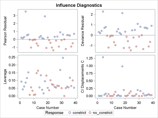
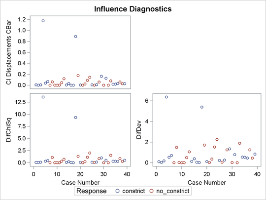
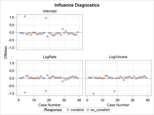
Because ODS Graphics is enabled, influence plots are displayed in Outputs Output 72.6.3 through Output 72.6.5. For general information about ODS Graphics, see Chapter 21: Statistical Graphics Using ODS. For specific information about the graphics available in the LOGISTIC procedure, see the section ODS Graphics. The vertical axis of an index plot represents the value of the diagnostic, and the horizontal axis represents the sequence (case number) of the observation. The index plots are useful for identification of extreme values.
The index plots of the Pearson residuals and the deviance residuals (Output 72.6.3) indicate that case 4 and case 18 are poorly accounted for by the model. The index plot of the diagonal elements of the hat matrix (Output 72.6.3) suggests that case 31 is an extreme point in the design space. The index plots of DFBETAS (Output 72.6.5) indicate that case 4 and case 18 are causing instability in all three parameter estimates. The other four index plots in Outputs Output 72.6.3 and Output 72.6.4 also point to these two cases as having a large impact on the coefficients and goodness of fit.
Output 72.6.3: Residuals, Hat Matrix, and CI Displacement C
Output 72.6.4: CI Displacement CBar, Change in Deviance and Pearson Chi-Square
Output 72.6.5: DFBETAS Plots
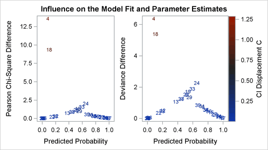
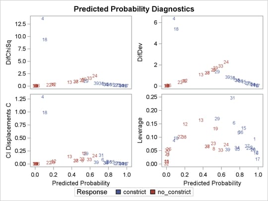
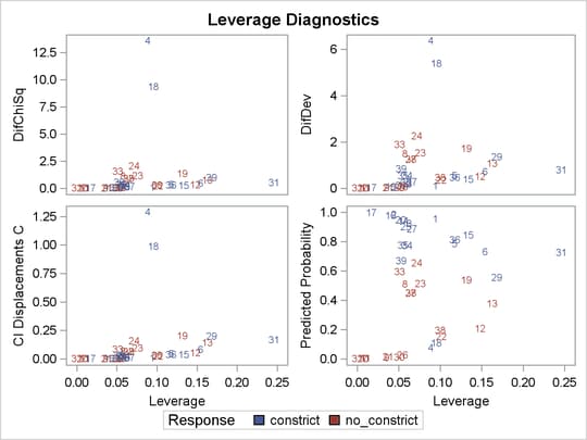
Other versions of diagnostic plots can be requested by specifying the appropriate options in the PLOTS= option. For example, the following statements produce three other sets of influence diagnostic plots: the PHAT option plots several diagnostics against the predicted probabilities (Output 72.6.6), the LEVERAGE option plots several diagnostics against the leverage (Output 72.6.7), and the DPC option plots the deletion diagnostics against the predicted probabilities and colors the observations according to the confidence interval displacement diagnostic (Output 72.6.8). The LABEL option displays the observation numbers on the plots. In all plots, you are looking for the outlying observations, and again cases 4 and 18 are noted.
proc logistic data=vaso plots(only label)=(phat leverage dpc);
   model Response=LogRate LogVolume;
run;
Output 72.6.6: Diagnostics versus Predicted Probability
Output 72.6.7: Diagnostics versus Leverage
Output 72.6.8: Three Diagnostics