The LOGISTIC Procedure
- Overview
- Getting Started
-
Syntax
 PROC LOGISTIC StatementBY StatementCLASS StatementCODE StatementCONTRAST StatementEFFECT StatementEFFECTPLOT StatementESTIMATE StatementEXACT StatementEXACTOPTIONS StatementFREQ StatementID StatementLSMEANS StatementLSMESTIMATE StatementMODEL StatementNLOPTIONS StatementODDSRATIO StatementOUTPUT StatementROC StatementROCCONTRAST StatementSCORE StatementSLICE StatementSTORE StatementSTRATA StatementTEST StatementUNITS StatementWEIGHT Statement
 -
DetailsMissing ValuesResponse Level OrderingLink Functions and the Corresponding DistributionsDetermining Observations for Likelihood ContributionsIterative Algorithms for Model FittingConvergence CriteriaExistence of Maximum Likelihood EstimatesEffect-Selection MethodsModel Fitting InformationGeneralized Coefficient of DeterminationScore Statistics and TestsConfidence Intervals for ParametersOdds Ratio EstimationRank Correlation of Observed Responses and Predicted ProbabilitiesLinear Predictor, Predicted Probability, and Confidence LimitsClassification TableOverdispersionThe Hosmer-Lemeshow Goodness-of-Fit TestReceiver Operating Characteristic CurvesTesting Linear Hypotheses about the Regression CoefficientsJoint Tests and Type 3 TestsRegression DiagnosticsScoring Data SetsConditional Logistic RegressionExact Conditional Logistic RegressionInput and Output Data SetsComputational ResourcesDisplayed OutputODS Table NamesODS Graphics
-
ExamplesStepwise Logistic Regression and Predicted ValuesLogistic Modeling with Categorical PredictorsOrdinal Logistic RegressionNominal Response Data: Generalized Logits ModelStratified SamplingLogistic Regression DiagnosticsROC Curve, Customized Odds Ratios, Goodness-of-Fit Statistics, R-Square, and Confidence LimitsComparing Receiver Operating Characteristic CurvesGoodness-of-Fit Tests and SubpopulationsOverdispersionConditional Logistic Regression for Matched Pairs DataExact Conditional Logistic RegressionFirth’s Penalized Likelihood Compared with Other ApproachesComplementary Log-Log Model for Infection RatesComplementary Log-Log Model for Interval-Censored Survival TimesScoring Data SetsUsing the LSMEANS StatementPartial Proportional Odds Model
- References
Exact Conditional Logistic Regression
The theory of exact logistic regression, also known as exact conditional logistic regression, was originally laid out by Cox (1970), and the computational methods employed in PROC LOGISTIC are described in Hirji, Mehta, and Patel (1987); Hirji (1992); Mehta, Patel, and Senchaudhuri (1992). Other useful references for the derivations include Cox and Snell (1989); Agresti (1990); Mehta and Patel (1995).
Exact conditional inference is based on generating the conditional distribution for the sufficient statistics of the parameters
of interest. This distribution is called the permutation or exact conditional distribution. Using the notation in the section Computational Details, follow Mehta and Patel (1995) and first note that the sufficient statistics  for the parameter vector of intercepts and slopes,
  , are
, are
![\[ T_ j = \sum _{i=1}^ n y_ ix_{ij}, \quad j=1,\ldots ,p \]](images/statug_logistic0667.png)
Denote a vector of observable sufficient statistics as  .
.
The probability density function (PDF) for  can be created by summing over all binary sequences
  that generate an observable
  and letting
  denote the number of sequences that generate
![\[ \Pr (\bT =\mb{t}) = \frac{C({\mb{t}})\exp ({\mb{t}}'\bbeta )}{\prod _{i=1}^ n[1+\exp (\mb{x}_ i'\bbeta )]} \]](images/statug_logistic0672.png)
In order to condition out the nuisance parameters, partition the parameter vector  , where
  is a
is a  vector of the nuisance parameters, and
  is the parameter vector for the remaining
  parameters of interest. Likewise, partition
  into
into  and
and  , into
  and
and  , and
, and  into
into  and
and  . The nuisance parameters can be removed from the analysis by conditioning on their sufficient statistics to create the conditional
likelihood of given
. The nuisance parameters can be removed from the analysis by conditioning on their sufficient statistics to create the conditional
likelihood of given  ,
,
where  is the number of vectors such that
  and
and  . Note that the nuisance parameters have factored out of this equation, and that
  is a constant.
The goal of the exact conditional analysis is to determine how likely the observed response  is with respect to all
  possible responses
  . One way to proceed is to generate every vector for which
  , and count the number of vectors for which
  is equal to each unique . Generating the conditional distribution from complete enumeration of the joint distribution is conceptually simple; however,
this method becomes computationally infeasible very quickly. For example, if you had only 30 observations, you would have
to scan through
is equal to each unique . Generating the conditional distribution from complete enumeration of the joint distribution is conceptually simple; however,
this method becomes computationally infeasible very quickly. For example, if you had only 30 observations, you would have
to scan through  different vectors.
Several algorithms are available in PROC LOGISTIC to generate the exact distribution. All of the algorithms are based on the
following observation. Given any  and a design
  , let
, let  and
and 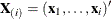 be the first i rows of each matrix. Write the sufficient statistic based on these i rows as
  . A recursion relation results:
 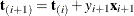 .
.
The following methods are available:
-
The multivariate shift algorithm developed by Hirji, Mehta, and Patel (1987), which steps through the recursion relation by adding one observation at a time and building an intermediate distribution at each step. If it determines that
 for the nuisance parameters could eventually equal , then is added to the intermediate distribution.
-
An extension of the multivariate shift algorithm to generalized logit models by Hirji (1992). Because the generalized logit model fits a new set of parameters to each logit, the number of parameters in the model can easily get too large for this algorithm to handle. Note for these models that the hypothesis tests for each effect are computed across the logit functions, while individual parameters are estimated for each logit function.
-
A network algorithm described in Mehta, Patel, and Senchaudhuri (1992), which builds a network for each parameter that you are conditioning out in order to identify feasible
 for the vector. These networks are combined and the set of feasible is further reduced, and then the multivariate shift algorithm uses this knowledge to build the exact distribution without
adding as many intermediate
for the vector. These networks are combined and the set of feasible is further reduced, and then the multivariate shift algorithm uses this knowledge to build the exact distribution without
adding as many intermediate  as the multivariate shift algorithm does.
-
A hybrid Monte Carlo and network algorithm described by Mehta, Patel, and Senchaudhuri (2000), which extends their 1992 algorithm by sampling from the combined network to build the exact distribution.
-
A Markov chain Monte Carlo algorithm described by Forster, McDonald, and Smith (2003), which generates the exact distribution by repeatedly perturbing the response vector to obtain a new response vector while maintaining the sufficient statistics for the nuisance parameters, and the resulting
are added to the exact distribution.
The bulk of the computation time and memory for these algorithms is consumed by the creation of the networks and the exact joint distribution. After the joint distribution for a set of effects is created, the computational effort required to produce hypothesis tests and parameter estimates for any subset of the effects is (relatively) trivial. See the section Computational Resources for Exact Logistic Regression for more computational notes about exact analyses.
Note: An alternative to using these exact conditional methods is to perform Firth’s bias-reducing penalized likelihood method (see the FIRTH option in the MODEL statement); this method has the advantage of being much faster and less memory intensive than exact algorithms, but it might not converge to a solution.
Hypothesis Tests
Consider testing the null hypothesis  against the alternative
  , conditional on
  . Under the null hypothesis, the test statistic for the exact probability test is just
  , while the corresponding p-value is the probability of getting a less likely (more extreme) statistic,
![\[ p(\mb{t}_\mr {I}|\mb{t}_\mr {N}) = \sum _{u\in \Omega _ p} f_{0}(\mb{u}|\mb{t}_\mr {N}) \]](images/statug_logistic0710.png)
where  there exist with
  , , and
 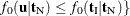 .
.
The exact probability test is not necessarily a sum of tail areas and can be inflated if the distribution is skewed. The more
robust exact conditional scores test is a sum of tail areas and is usually preferred to the exact probability test. To compute the exact conditional scores test,
the conditional mean  and variance matrix
  of the (conditional on ) are calculated, and the score statistic for the observed value,
![\[ s = (\mb{t}_\mr {I}-\bmu _\mr {I})’\bSigma _\mr {I}^{-1}(\mb{t}_\mr {I}-\bmu _\mr {I}) \]](images/statug_logistic0716.png)
is compared to the score for each member of the distribution
![\[ S(\bT _\mr {I}) = (\bT _\mr {I}-\bmu _\mr {I})’\bSigma _\mr {I}^{-1}(\bT _\mr {I}-\bmu _\mr {I}) \]](images/statug_logistic0717.png)
The resulting p-value is
![\[ p(\mb{t}_\mr {I}|\mb{t}_\mr {N}) = \Pr (S\ge s) = \sum _{u\in \Omega _ s} f_{0}(\mb{u}|\mb{t}_\mr {N}) \]](images/statug_logistic0718.png)
where  there exist with , , and
  .
.
The mid-p statistic, defined as
![\[ p(\mb{t}_\mr {I}|\mb{t}_\mr {N})- \frac{1}{2}f_{0}(\mb{t}_\mr {I}|\mb{t}_\mr {N}) \]](images/statug_logistic0721.png)
was proposed by Lancaster (1961) to compensate for the discreteness of a distribution. See Agresti (1992) for more information. However, to allow for more flexibility in handling ties, you can write the mid-p statistic as (based on a suggestion by LaMotte (2002) and generalizing Vollset, Hirji, and Afifi (1991))
![\[ \sum _{u\in \Omega _<} f_{0}(\mb{u}|\mb{t}_\mr {N}) + \delta _1 f_{0}(\mb{t}_\mr {I}|\mb{t}_\mr {N}) + \delta _2 \sum _{u\in \Omega _=} f_{0}(\mb{u}|\mb{t}_\mr {N}) \]](images/statug_logistic0722.png)
where, for  ,
,  is
is  using strict inequalities, and
  is using equalities with the added restriction that
  . Letting
  yields Lancaster’s mid-p.
Caution: When the exact distribution has ties and you specify METHOD=NETWORKMC
or METHOD=MCMC
, the sampling algorithm estimates  with error, and hence it cannot determine precisely which values contribute to the reported p-values. For example, if the exact distribution has densities
  and if the observed statistic has probability 0.2, then the exact probability p-value is exactly 0.6. Under Monte Carlo sampling, if the densities after N samples are
  and the observed probability is 0.21, then the resulting p-value is 0.39. Therefore, the exact probability test p-value for this example fluctuates between 0.2, 0.4, and 0.6, and the reported p-values are actually lower bounds for the true p-values. If you need more precise values, you can specify the OUTDIST=
option, determine appropriate cutoff values for the observed probability and score, and then construct p-value estimates from the OUTDIST= data set and display them in the SAS log by using the following statements:
and the observed probability is 0.21, then the resulting p-value is 0.39. Therefore, the exact probability test p-value for this example fluctuates between 0.2, 0.4, and 0.6, and the reported p-values are actually lower bounds for the true p-values. If you need more precise values, you can specify the OUTDIST=
option, determine appropriate cutoff values for the observed probability and score, and then construct p-value estimates from the OUTDIST= data set and display them in the SAS log by using the following statements:
data _null_;
   set outdist end=end;
   retain pvalueProb 0 pvalueScore 0;
   if prob < ProbCutOff then pvalueProb+prob;
   if score > ScoreCutOff then pvalueScore+prob;
   if end then put pvalueProb= pvalueScore=;
run;
Because the METHOD=MCMC samples are correlated, the covariance that is computed for the exact conditional scores test is biased. Specifying the NTHIN= option might reduce this bias.
Inference for a Single Parameter
Exact parameter estimates are derived for a single parameter  by regarding all the other parameters
  as nuisance parameters. The appropriate sufficient statistics are
  and
and  , with their observed values denoted by the lowercase t. Hence, the conditional PDF used to create the parameter estimate for is
![\[ f_{\beta _ i}(t_ i|\mb{t}_\mr {N}) = \frac{C(\mb{t}_\mr {N},t_ i)\exp (t_ i\beta _ i)}{\sum _{u\in \Omega }C(\mb{t}_\mr {N},u)\exp (u\beta _ i)} \]](images/statug_logistic0735.png)
for  .
.
The maximum exact conditional likelihood estimate is the quantity  , which maximizes the conditional PDF. A Newton-Raphson algorithm is used to perform this search. However, if the observed
 attains either its maximum or minimum value in the exact distribution (that is, either
  or
or  ), then the conditional PDF is monotonically increasing in and cannot be maximized. In this case, a median unbiased estimate (Hirji, Tsiatis, and Mehta 1989) is produced that satisfies
  , and a Newton-Raphson algorithm is used to perform the search.
The standard error of the exact conditional likelihood estimate is just the negative of the inverse of the second derivative of the exact conditional log likelihood (Agresti 2002).
Likelihood ratio tests based on the conditional PDF are used to test the null  against the alternative
  . The critical region for this UMP test consists of the upper tail of values for
  in the exact distribution. Thus, the p-value
  for a one-tailed test is
![\[ p_+(t_ i;0) = \sum _{u\ge t_ i}f_{0}(u|\mb{t}_\mr {N}) \]](images/statug_logistic0746.png)
Similarly, the p-value  for the one-tailed test of
  against
  is
is
![\[ p_-(t_ i;0) = \sum _{u\le t_ i}f_{0}(u|\mb{t}_\mr {N}) \]](images/statug_logistic0749.png)
The p-value  for a two-tailed test of against
  is
is
![\[ p(t_ i;0) = 2\min [p_-(t_ i;0),p_+(t_ i;0)] \]](images/statug_logistic0752.png)
The p-value that is reported for a single parameter in the "Exact Parameter Estimates" table is for the two-tailed test.
An upper  % exact confidence limit for corresponding to the observed is the solution
  of
of 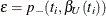 , while the lower exact confidence limit is the solution
  of
of 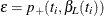 . Again, a Newton-Raphson procedure is used to search for the solutions. Note that one of the confidence limits for a median
unbiased estimate is set to infinity, but the other is still computed at
. Again, a Newton-Raphson procedure is used to search for the solutions. Note that one of the confidence limits for a median
unbiased estimate is set to infinity, but the other is still computed at  . This results in the display of a one-sided
  % confidence interval; if you want the
  limit instead, you can specify the ONESIDED
option.
limit instead, you can specify the ONESIDED
option.
Specifying the ONESIDED
option displays only one p-value and one confidence interval, because small values of and support different alternative hypotheses and only one of these p-values can be less than 0.50.
The mid-p confidence limits are the solutions to  for
for 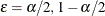 (Vollset, Hirji, and Afifi 1991).
  produces the usual exact (or max-p) confidence interval,
  yields the mid-p interval, and
  gives the min-p interval. The mean of the endpoints of the max-p and min-p intervals provides the mean-p interval as defined by Hirji, Mehta, and Patel (1988).
Estimates and confidence intervals for the odds ratios are produced by exponentiating the estimates and interval endpoints for the parameters.