The LOGISTIC Procedure
- Overview
- Getting Started
-
Syntax
 PROC LOGISTIC StatementBY StatementCLASS StatementCODE StatementCONTRAST StatementEFFECT StatementEFFECTPLOT StatementESTIMATE StatementEXACT StatementEXACTOPTIONS StatementFREQ StatementID StatementLSMEANS StatementLSMESTIMATE StatementMODEL StatementNLOPTIONS StatementODDSRATIO StatementOUTPUT StatementROC StatementROCCONTRAST StatementSCORE StatementSLICE StatementSTORE StatementSTRATA StatementTEST StatementUNITS StatementWEIGHT Statement
 -
DetailsMissing ValuesResponse Level OrderingLink Functions and the Corresponding DistributionsDetermining Observations for Likelihood ContributionsIterative Algorithms for Model FittingConvergence CriteriaExistence of Maximum Likelihood EstimatesEffect-Selection MethodsModel Fitting InformationGeneralized Coefficient of DeterminationScore Statistics and TestsConfidence Intervals for ParametersOdds Ratio EstimationRank Correlation of Observed Responses and Predicted ProbabilitiesLinear Predictor, Predicted Probability, and Confidence LimitsClassification TableOverdispersionThe Hosmer-Lemeshow Goodness-of-Fit TestReceiver Operating Characteristic CurvesTesting Linear Hypotheses about the Regression CoefficientsJoint Tests and Type 3 TestsRegression DiagnosticsScoring Data SetsConditional Logistic RegressionExact Conditional Logistic RegressionInput and Output Data SetsComputational ResourcesDisplayed OutputODS Table NamesODS Graphics
-
ExamplesStepwise Logistic Regression and Predicted ValuesLogistic Modeling with Categorical PredictorsOrdinal Logistic RegressionNominal Response Data: Generalized Logits ModelStratified SamplingLogistic Regression DiagnosticsROC Curve, Customized Odds Ratios, Goodness-of-Fit Statistics, R-Square, and Confidence LimitsComparing Receiver Operating Characteristic CurvesGoodness-of-Fit Tests and SubpopulationsOverdispersionConditional Logistic Regression for Matched Pairs DataExact Conditional Logistic RegressionFirth’s Penalized Likelihood Compared with Other ApproachesComplementary Log-Log Model for Infection RatesComplementary Log-Log Model for Interval-Censored Survival TimesScoring Data SetsUsing the LSMEANS StatementPartial Proportional Odds Model
- References
Score Statistics and Tests
To understand the general form of the score statistics, let  be the vector of first partial derivatives of the log likelihood with respect to the parameter vector
  , and let
  be the matrix of second partial derivatives of the log likelihood with respect to .
That is, is the gradient vector, and is the Hessian matrix.
Let
be the matrix of second partial derivatives of the log likelihood with respect to .
That is, is the gradient vector, and is the Hessian matrix.
Let  be either
  or the expected value of . Consider a null hypothesis
  . Let
. Let  be the MLE of under . The chi-square score statistic for testing is defined by
![\[ \mb{g}’({\widehat{\bbeta }}_{H_0})\bI ^{-1}({\widehat{\bbeta }}_{H_0})\mb{g} ({\widehat{\bbeta }}_{H_0}) \]](images/statug_logistic0246.png)
and it has an asymptotic  distribution with r degrees of freedom under , where r is the number of restrictions imposed on by .
Residual Chi-Square
When you use SELECTION= FORWARD, BACKWARD, or STEPWISE, the procedure calculates a residual chi-square score statistic and reports the statistic, its degrees of freedom, and the p-value. This section describes how the statistic is calculated.
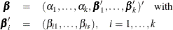
Suppose there are s explanatory effects of interest. The full cumulative response model has a parameter vector
![\[ \bbeta =(\alpha _{1},\ldots ,\alpha _{k},\beta _1,\ldots ,\beta _ s)’ \]](images/statug_logistic0248.png)
where  are intercept parameters, and
  are the common slope parameters for the s explanatory effects. The full generalized logit model has a parameter vector
where  is the slope parameter for the jth effect in the ith logit.
Consider the null hypothesis 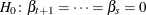 , where
  for the cumulative response model, and
  , for the generalized logit model. For the reduced model with t explanatory effects, let
  be the MLEs of the unknown intercept parameters, let
  be the MLEs of the unknown slope parameters, and let
 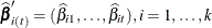 , be those for the generalized logit model. The residual chi-square is the chi-square score statistic testing the null hypothesis
; that is, the residual chi-square is
, be those for the generalized logit model. The residual chi-square is the chi-square score statistic testing the null hypothesis
; that is, the residual chi-square is
where for the cumulative response model  , and for the generalized logit model
  , where
  denotes a vector of
  zeros.
The residual chi-square has an asymptotic chi-square distribution with degrees of freedom ( for the generalized logit model). A special case is the global score chi-square, where the reduced model consists of the
k intercepts and no explanatory effects. The global score statistic is displayed in the "Testing Global Null Hypothesis: BETA=0"
table. The table is not produced when the NOFIT
option is used, but the global score statistic is displayed.
for the generalized logit model). A special case is the global score chi-square, where the reduced model consists of the
k intercepts and no explanatory effects. The global score statistic is displayed in the "Testing Global Null Hypothesis: BETA=0"
table. The table is not produced when the NOFIT
option is used, but the global score statistic is displayed.
Testing Individual Effects Not in the Model
These tests are performed when you specify SELECTION= FORWARD or STEPWISE, and are displayed when the DETAILS option is specified. In the displayed output, the tests are labeled "Score Chi-Square" in the "Analysis of Effects Eligible for Entry" table and in the "Summary of Stepwise (Forward) Selection" table. This section describes how the tests are calculated.
Suppose that k intercepts and t explanatory variables (say  ) have been fit to a model and that
  is another explanatory variable of interest. Consider a full model with the k intercepts and
  explanatory variables (
 ) and a reduced model with excluded. The significance of adjusted for
  can be determined by comparing the corresponding residual chi-square with a chi-square distribution with one degree of freedom
(k degrees of freedom for the generalized logit model).
can be determined by comparing the corresponding residual chi-square with a chi-square distribution with one degree of freedom
(k degrees of freedom for the generalized logit model).
Testing the Parallel Lines Assumption
For an ordinal response, PROC LOGISTIC performs a test of the parallel lines assumption. In the displayed output, this test is labeled "Score Test for the Equal Slopes Assumption" when the LINK= option is NORMIT or CLOGLOG. When LINK=LOGIT, the test is labeled as "Score Test for the Proportional Odds Assumption" in the output. For small sample sizes, this test might be too liberal (Stokes, Davis, and Koch 2000, p. 249). This section describes the methods used to calculate the test.
For this test the number of response levels,  , is assumed to be strictly greater than 2. Let Y be the response variable taking values
  . Suppose there are s explanatory variables. Consider the general cumulative model without making the parallel lines assumption
![\[ g(\mbox{Pr}(Y\leq i~ |~ \mb{x}))= (1,\mb{x}’)\bbeta _ i, \quad 1 \leq i \leq k \]](images/statug_logistic0268.png)
where  is the link function, and
 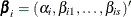 is a vector of unknown parameters consisting of an intercept
  and s slope parameters
  . The parameter vector for this general cumulative model is
![\[ \bbeta =(\bbeta ’_1,\ldots ,\bbeta ’_ k)’ \]](images/statug_logistic0273.png)
Under the null hypothesis of parallelism  , there is a single common slope parameter for each of the s explanatory variables. Let
  be the common slope parameters. Let and
  be the MLEs of the intercept parameters and the common slope parameters. Then, under , the MLE of is
![\[ {\widehat{\bbeta }_{H_0}}=({\widehat{\bbeta }}’_1,\ldots ,{\widehat{\bbeta }}’_ k)’ \quad \mbox{with} \quad {\widehat{\bbeta }}_ i=({\widehat{\alpha }_{i}},{\widehat{\beta }}_1,\ldots , {\widehat{\beta }}_ s)’ \quad 1 \leq i \leq k \]](images/statug_logistic0277.png)
and the chi-square score statistic  has an asymptotic chi-square distribution with
  degrees of freedom. This tests the parallel lines assumption by testing the equality of separate slope parameters simultaneously
for all explanatory variables.
degrees of freedom. This tests the parallel lines assumption by testing the equality of separate slope parameters simultaneously
for all explanatory variables.