The HPMIXED Procedure

PROC HPMIXED Statement
-
PROC HPMIXED <options>;
The PROC HPMIXED statement invokes the HPMIXED procedure. Table 55.2 summarizes the options available in the PROC HPMIXED statement. These and other options in the PROC HPMIXED statement are then described fully in alphabetical order.
Table 55.2: PROC HPMIXED Statement Options
|
Option |
Description |
|---|---|
|
Basic Options |
|
|
Specifies input data set |
|
|
Specifies the estimation method |
|
|
Includes scale parameter in optimization |
|
|
Determines the sort order of CLASS variables |
|
|
Computes BLUP/BLUE only |
|
|
Displayed Output |
|
|
Displays a table of information criteria |
|
|
Displays estimates and gradients added to "Iteration History" |
|
|
Specifies the maximum levels of CLASS variables to print |
|
|
Writes periodic status notes to the log |
|
|
Displays mixed model equations |
|
|
Suppresses "Class Level Information" completely or in parts |
|
|
Suppresses "Iteration History" table |
|
|
Displays a table of ranks of matrices |
|
|
Displays "Descriptive Statistics" table |
|
|
Singularity Tolerances |
|
|
Tunes singularity for Cholesky decompositions |
|
|
Tunes singularity for the residual variance |
|
|
Tunes general singularity criterion |
|
You can specify the following options.
- BLUP<(suboptions)>=SAS-data-set
-
creates a data set that contains the BLUE and BLUP solutions.The covariance parameters are assumed to be known and given by PARMS statement. All hypothesis testing is ignored. The statements TEST, ESTIMATE, CONTRAST, LSMEANS, and OUTPUT are all ignored. This option is designed for users who need BLUP solutions for random effects with many levels, up to tens of millions.
You can specify the following suboptions:
- ITPRINT=number
-
specifies that the iteration history be displayed after every number of iterations. This suboption applies only for iterative solving methods (IOC or IOD). The default value is 10, which means the procedure displays the iteration history for every 10 iterations.
- MAXITER=number
-
specifies the maximum number of iterations allowed. This applies only for iterative solving methods (IOC or IOD). The default value is the number of parameters in the BLUE/BLUP plus two.
- METHOD=DIRECT | IOC | IOD
-
specifies the method used to solve for BLUP solutions. METHOD=DIRECT requires storing mixed model equations (MMEQ) in memory and computing the Cholesky decomposition of MMEQ. This method is the most accurate, but it is the most inefficient in terms of speed and memory. METHOD=IOD does not build mixed model equations; instead it iterates on data to solve for the solutions. This method is most efficient in terms of memory. METHOD=IOC requires storing mixed model equations in memory and iterates on MMEQ to solve for the solutions. This method is the most efficient in terms of speed. The default method is IOC.
- TOL=number
-
specifies the tolerance value. This suboption applies only for iterative solving methods (IOC or IOD). The default value is the square root of machine precision.
- DATA=SAS-data-set
-
names the SAS data set to be used by PROC HPMIXED. The default is the most recently created data set.
-
INFOCRIT=NONE | PQ | Q
IC=NONE | PQ | Q -
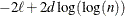
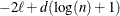
determines the computation of information criteria in the "Fit Statistics" table. The criteria are all in smaller-is-better form, and are described in Table 55.3.
Table 55.3: Information Criteria
Here
 denotes the maximum value of the restricted log likelihood, d is the dimension of the model, and n,
  reflect the size of the data. When
  , the value of the HQIC criterion is
  . When n=0, the values of the BIC and CAIC criteria are undefined.
The quantities d, n, and
depend on the model and IC= option.
-
models without random effects: The IC=Q and IC=PQ options have no effect on the computation.
-
d equals the number of parameters in the optimization whose solutions do not fall on the boundary or are otherwise constrained.
-
n equals the number of used observations minus rank(X).
-
equals n, unless n < d + 2, in which case
 .
.
-
-
models with random effects:
-
d equals the number of parameters in the optimization whose solutions do not fall on the boundary or are otherwise constrained. If IC=PQ, this value is incremented by
 .
.
-
n equals the effective number of subjects as displayed in the "Dimensions" table, unless this value equals 1, in which case n equals the number of levels of the first random effect specified. The IC=Q and IC=PQ options have no effect.
-
equals n, unless n < d + 2, in which case . The IC=Q and IC=PQ options have no effect.
-
The IC=NONE option suppresses the "Fit Statistics" table. IC=Q is the default.
-
- ITDETAILS
-
displays the parameter values at each iteration and enables the writing of notes to the SAS log pertaining to "infinite likelihood" and "singularities" during optimization iterations.
- LOGNOTE
-
writes to the log periodic notes that describe the current status of computations. This option is designed for use with analyses that require extensive CPU resources.
- MAXCLPRINT=number
-
specifies the maximum levels of CLASS variables to print in the ODS table ClassLevels. The default value is 20. MAXCLPRINT=0 enables you to print all levels of each CLASS variable. However, the option NOCLPRINT takes precedence over MAXCLPRINT.
- METHOD=
-
specifies the estimation method for the covariance parameters. The REML specification performs residual (restricted) maximum likelihood, and it is currently the only available method. This option is therefore currently redundant for PROC HPMIXED, but it is included for consistency with other mixed model procedures in SAS/STAT software.
- MMEQ
-
displays coefficients of the mixed model equations. These are
![\[ \left[\begin{array}{lr} \bX ’\widehat{\bR }^{-1}\bX & \bX ’\widehat{\bR }^{-1}\bZ \\*\bZ ’\widehat{\bR }^{-1}\bX & \bZ ’\widehat{\bR }^{-1} \bZ + \widehat{\bG }^{-1} \end{array}\right] \left[\begin{array}{c} \bX ’\widehat{\bR }^{-1}\mb{y} \\ \bZ ’\widehat{\bR }^{-1}\mb{y} \end{array} \right] \]](images/statug_hpmixed0040.png)
assuming
 is nonsingular. If is singular, PROC HPMIXED produces the following coefficients
![\[ \left[\begin{array}{lr} \bX ’\widehat{\bR }^{-1}\bX & \bX ’\widehat{\bR }^{-1}\bZ \widehat{\bG }\\*\widehat{\bG } \bZ ’\widehat{\bR }^{-1}\bX & \widehat{\bG } \bZ ’\widehat{\bR }^{-1}\bZ \widehat{\bG } + \widehat{\bG } \end{array}\right] \left[\begin{array}{c} \bX ’\widehat{\bR }^{-1}\mb{y} \\ \widehat{\bG } \bZ ’\widehat{\bR }^{-1}\mb{y} \end{array} \right] \]](images/statug_hpmixed0042.png)
See the section "Model and Assumptions" for further information about these equations.
- NAMELEN=number
-
specifies the length to which long effect names are shortened. The default and minimum value is 20.
- NLPRINT
-
requests that optimization-related output options specified in the NLOPTIONS statement override corresponding options in the PROC HPMIXED statement. When you specify NLPRINT, the ITDETAILS and NOITPRINT options in the PROC HPMIXED statement are ignored and the following six options in the NLOPTIONS statement are enabled: NOPRINT, PHISTORY, PSUMMARY, PALL, PLONG, and PHISTPARMS.
The syntax and options of the NLOPTIONS statement are described in the section NLOPTIONS Statement in Chapter 19: Shared Concepts and Topics.
- NOCLPRINT<=number>
-
suppresses the display of the "Class Level Information" table if you do not specify number. If you do specify number, only levels with totals that are less than number are listed in the table.
- NOFIT
-
suppresses fitting of the model. When the NOFIT option is in effect, PROC HPMIXED produces the "Model Information," "Class Level Information," "Number of Observations," "Dimensions," and "Descriptive Statistics" tables. These can be helpful in gauging the computational effort required to fit the model.
- NOINFO
-
suppresses the display of the "Model Information," "Number of Observations," and "Dimensions" tables.
- NOITPRINT
- NOPRINT
-
suppresses the normal display of results. The NOPRINT option is useful when you want only to create one or more output data sets with the procedure by using the OUTPUT statement. Note that this option temporarily disables the Output Delivery System (ODS); see Chapter 20: Using the Output Delivery System, for more information.
- NOPROFILE
-
includes the residual variance as one of the covariance parameters in the optimization iterations. This option applies only to models that have a residual variance parameter. By default, this parameter is profiled out of the optimization iterations, except when you have specified the HOLD= option in the PARMS statement.
- ORDER=DATA | FORMATTED | FREQ | INTERNAL
-
specifies the sort order for the levels of the classification variables (which are specified in the CLASS statement).
This option applies to the levels for all classification variables, except when you use the (default) ORDER=FORMATTED option with numeric classification variables that have no explicit format. In that case, the levels of such variables are ordered by their internal value.
The ORDER= option can take the following values:
Value of ORDER=
Levels Sorted By
DATA
Order of appearance in the input data set
FORMATTED
External formatted value, except for numeric variables with no explicit format, which are sorted by their unformatted (internal) value
FREQ
Descending frequency count; levels with the most observations come first in the order
INTERNAL
Unformatted value
By default, ORDER=FORMATTED. For ORDER=FORMATTED and ORDER=INTERNAL, the sort order is machine-dependent.
For more information about sort order, see the chapter on the SORT procedure in the Base SAS Procedures Guide and the discussion of BY-group processing in SAS Language Reference: Concepts.
- RANKS
-
displays the ranks of design matrices
 and (
and ( ) and the coefficient matrix of the mixed model equations (
 ).
).
- SIMPLE
-
displays the mean, standard deviation, coefficient of variation, minimum, and maximum for each variable used in PROC HPMIXED that is not a classification variable.
- SINGCHOL=number
-
tunes the singularity criterion in Cholesky decompositions. The default is 1E6 times the machine epsilon; this product is approximately 1E–10 on most computers.
- SINGRES=number
-
sets the tolerance for which the residual variance is considered to be zero. The default is 1E4 times the machine epsilon; this product is approximately 1E–12 on most computers.
- SINGULAR=number
-
tunes the general singularity criterion applied by the HPMIXED procedure in divisions and inversions. The default is 1E4 times the machine epsilon; this product is approximately 1E–12 on most computers.
- UPDATE
-
is an alias for the LOGNOTE option.