The HPMIXED Procedure

The HPMIXED procedure handles only a subset of the analyses of the GLIMMIX procedure. However, you can use the HPMIXED procedure to accelerate your GLIMMIX procedure analyses for large problems. The idea is to use PROC HPMIXED to maximize the likelihood and produce parameter estimates more quickly than PROC GLIMMIX, and then to pass these parameter estimates to PROC GLIMMIX for some further analysis that is not available within PROC HPMIXED.

This example revisits the mixed model problem from the section Getting Started: HPMIXED Procedure to illustrate how to obtain the covariance estimates from the HPMIXED procedure and, in turn, how to use these estimates in PROC GLIMMIX’s PARMS statement. The following statements again simulate data from animals of different species on different farms:

data Sim;
   keep Species Farm Animal Yield;
   array AnimalEffect{3000};
   array AnimalSpecies{3000};
   array AnimalFarm{3000};
   do i = 1 to 3000;
      AnimalEffect{i} = sqrt(4.0)*rannor(12345);
      AnimalSpecies{i} = 1 + int(5*ranuni(12345));
      AnimalFarm{i}    = 1 + int(10*ranuni(12345));
   end;
   do i = 1 to 40000;
      Animal  = 1 + int(3000*ranuni(12345));
      Species = AnimalSpecies{Animal};
      Farm    = AnimalFarm{Animal};
      Yield   = 1 + Species + int(Farm/2) + AnimalEffect{Animal}
                  + sqrt(8.0)*rannor(12345);
      output;
   end;
run;

Note that in the preceding DATA step program, certain pairs of farms are simulated to have the same effect on yield. Suppose that your goal is to determine which farms are significantly different. While the HPMIXED procedure has an LSMEANS statement, it has no options for multiple comparisons. The following statements first use the HPMIXED procedure to obtain the covariance estimates, saving them in the SAS data set HPMEstimate. Then the GLIMMIX procedure is executed with the PARMS statement to initialize the parameter values from the data set HPMEstimate and with the HOLD= and NOITER options to prevent further optimization iterations. The LSMEANS statement is used in PROC GLIMMIX to perform multiple comparisons of the LS-means for farms, and the results are displayed as a so-called diffogram.

proc hpmixed data=Sim;
   class Species Farm Animal;
   model Yield = Farm|Species;
   random Animal;
   test Species Species*Farm;
   ods output CovParms=HPMEstimate;
run;

ods graphics on;
proc glimmix data=Sim;
   class Species Farm Animal;
   model Yield = Farm|Species;
   random int/sub=Animal;
   parms /pdata=HPMEstimate hold=1,2 noiter;
   lsmeans Farm / pdiff=all plot=diffplot;
run;

The iteration histories for the two procedures are shown in Output 55.3.1 and Output 55.3.2. Whereas PROC HPMIXED requires several iterations in order to converge, PROC GLIMMIX "converges" to the same value in one step, with no iteration since the options HOLD= and NOITER are used.

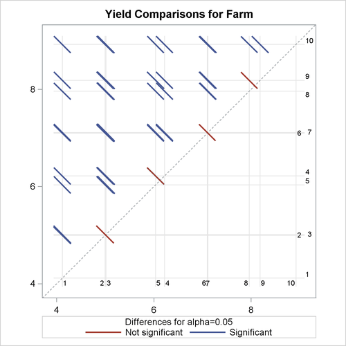
The graphical multiple-comparisons analysis for the LS-means of farms is shown in Output 55.3.3. It confirms the pairwise equalities between farm effects with which the data were simulated.

Output 55.3.3: LS-Means Plot of Pairwise Farm Differences

For more information about the interpretation of the LS-means difference plot, see the section ODS Graphics, in Chapter 45: The GLIMMIX Procedure.