The UNIVARIATE Procedure
- Overview
-
Getting Started

-
Syntax
-
DetailsMissing ValuesRoundingDescriptive StatisticsCalculating the ModeCalculating PercentilesTests for LocationConfidence Limits for Parameters of the Normal DistributionRobust EstimatorsCreating Line Printer PlotsCreating High-Resolution GraphicsUsing the CLASS Statement to Create Comparative PlotsPositioning InsetsFormulas for Fitted Continuous DistributionsGoodness-of-Fit TestsKernel Density EstimatesConstruction of Quantile-Quantile and Probability PlotsInterpretation of Quantile-Quantile and Probability PlotsDistributions for Probability and Q-Q PlotsEstimating Shape Parameters Using Q-Q PlotsEstimating Location and Scale Parameters Using Q-Q PlotsEstimating Percentiles Using Q-Q PlotsInput Data SetsOUT= Output Data Set in the OUTPUT StatementOUTHISTOGRAM= Output Data SetOUTKERNEL= Output Data SetOUTTABLE= Output Data SetTables for Summary StatisticsODS Table NamesODS Tables for Fitted DistributionsODS GraphicsComputational Resources
-
ExamplesComputing Descriptive Statistics for Multiple VariablesCalculating ModesIdentifying Extreme Observations and Extreme ValuesCreating a Frequency TableCreating Basic Summary PlotsAnalyzing a Data Set With a FREQ VariableSaving Summary Statistics in an OUT= Output Data SetSaving Percentiles in an Output Data SetComputing Confidence Limits for the Mean, Standard Deviation, and VarianceComputing Confidence Limits for Quantiles and PercentilesComputing Robust EstimatesTesting for LocationPerforming a Sign Test Using Paired DataCreating a HistogramCreating a One-Way Comparative HistogramCreating a Two-Way Comparative HistogramAdding Insets with Descriptive StatisticsBinning a HistogramAdding a Normal Curve to a HistogramAdding Fitted Normal Curves to a Comparative HistogramFitting a Beta CurveFitting Lognormal, Weibull, and Gamma CurvesComputing Kernel Density EstimatesFitting a Three-Parameter Lognormal CurveAnnotating a Folded Normal CurveCreating Lognormal Probability PlotsCreating a Histogram to Display Lognormal FitCreating a Normal Quantile PlotAdding a Distribution Reference LineInterpreting a Normal Quantile PlotEstimating Three Parameters from Lognormal Quantile PlotsEstimating Percentiles from Lognormal Quantile PlotsEstimating Parameters from Lognormal Quantile PlotsComparing Weibull Quantile PlotsCreating a Cumulative Distribution PlotCreating a P-P Plot
- References
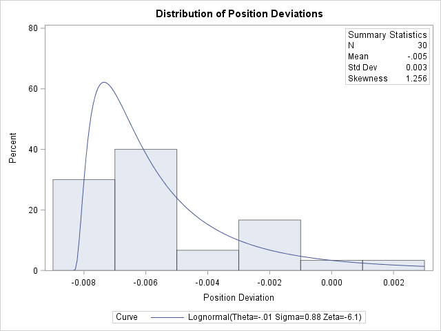
Example 4.27 Creating a Histogram to Display Lognormal Fit
This example uses the data set Aircraft from Example 4.26 to illustrate how to display a lognormal fit with a histogram. To determine whether the lognormal distribution is an appropriate
model for a distribution, you should consider the graphical fit as well as conduct goodness-of-fit tests. The following statements
fit a lognormal distribution and display the density curve on a histogram:
title 'Distribution of Position Deviations';
ods select Histogram Lognormal.ParameterEstimates Lognormal.GoodnessOfFit;
proc univariate data=Aircraft;
   var Deviation;
   histogram / lognormal(w=3 theta=est)
               odstitle = title;
   inset n mean (5.3) std='Std Dev' (5.3) skewness (5.3) /
      pos    = ne
      header = 'Summary Statistics';
run;
The ODS SELECT statement restricts the output to the "ParameterEstimates" and "GoodnessOfFit" tables; see the section ODS Table Names. The LOGNORMAL primary option superimposes a fitted curve on the histogram in Output 4.27.1. The W= option specifies the line width for the curve. The INSET statement specifies that the mean, standard deviation, and
skewness be displayed in an inset in the northeast corner of the plot. Note that the default value of the threshold parameter
is zero. In applications where the threshold is not zero, you can specify with the THETA= option. The variable Deviation includes values that are less than the default threshold; therefore, the option THETA= EST is used.
Output 4.27.1: Normal Probability Plot Created with Graphics Device
Output 4.27.2 provides three EDF goodness-of-fit tests for the lognormal distribution: the Anderson-Darling, the Cramér–von Mises, and
the Kolmogorov-Smirnov tests. The null hypothesis for the three tests is that a lognormal distribution holds for the sample
data.
Output 4.27.2: Summary of Fitted Lognormal Distribution
The p-values for all three tests are greater than 0.5, so the null hypothesis is not rejected. The tests support the conclusion that the two-parameter lognormal distribution with scale parameter and shape parameter provides a good model for the distribution of position deviations. For further discussion of goodness-of-fit interpretation, see the section Goodness-of-Fit Tests.
A sample program for this example, uniex16.sas, is available in the SAS Sample Library for Base SAS software.