The UNIVARIATE Procedure

You can use a beta distribution to model the distribution of a variable that is known to vary between lower and upper bounds. In this example, a manufacturing company uses a robotic arm to attach hinges on metal sheets. The attachment point should be offset 10.1 mm from the left edge of the sheet. The actual offset varies between 10.0 and 10.5 mm due to variation in the arm. The following statements save the offsets for 50 attachment points as the values of the variable Length in the data set Robots:

data Robots;
   input Length @@;
   label Length = 'Attachment Point Offset (in mm)';
   datalines;
10.147 10.070 10.032 10.042 10.102
10.034 10.143 10.278 10.114 10.127
10.122 10.018 10.271 10.293 10.136
10.240 10.205 10.186 10.186 10.080
10.158 10.114 10.018 10.201 10.065
10.061 10.133 10.153 10.201 10.109
10.122 10.139 10.090 10.136 10.066
10.074 10.175 10.052 10.059 10.077
10.211 10.122 10.031 10.322 10.187
10.094 10.067 10.094 10.051 10.174
;

The following statements create a histogram with a fitted beta density curve, shown in Output 4.21.1:

ods select ParameterEstimates FitQuantiles Histogram;
proc univariate data=Robots;
   histogram Length /
      beta(theta=10 scale=0.5 fill)
      href      = 10
      hreflabel = 'Lower Bound'
      odstitle  = 'Fitted Beta Distribution of Offsets';
   inset n = 'Sample Size' /
      pos=ne  cfill=blank;
run;

The ODS SELECT statement restricts the output to the "ParameterEstimates" and "FitQuantiles" tables and the histogram; see the section ODS Table Names. The BETA primary option requests a fitted beta distribution. The THETA= secondary option specifies the lower threshold. The SCALE= secondary option specifies the range between the lower threshold and the upper threshold. Note that the default THETA= and SCALE= values are zero and one, respectively.

Output 4.21.1: Superimposing a Histogram with a Fitted Beta Curve

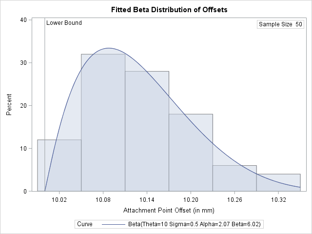
The FILL secondary option specifies that the area under the curve is to be filled. The HREF= option draws a reference line at the lower bound, and the HREFLABEL= option adds the label Lower Bound. The ODSTITLE= option adds a title to the histogram. The INSET statement adds an inset with the sample size positioned in the northeast corner of the plot.

In addition to displaying the beta curve, the BETA option requests a summary of the curve fit. This summary, which includes parameters for the curve and the observed and estimated quantiles, is shown in Output 4.21.2.

A sample program for this example, uniex12.sas, is available in the SAS Sample Library for Base SAS software.