The HPPANEL Procedure
- Overview
- Getting Started
-
Syntax

-
DetailsSpecifying the Input DataSpecifying the Regression ModelSpecifying the Number of Nodes and Number of ThreadsUnbalanced DataOne-Way Fixed-Effects ModelTwo-Way Fixed-Effects ModelBalanced PanelsUnbalanced PanelsOne-Way Random-Effects ModelTwo-Way Random-Effects ModelBetween EstimatorsPooled EstimatorLinear Hypothesis TestingSpecification TestsOUTPUT OUT= Data SetOUTEST= Data SetPrinted OutputODS Table Names
-
Example
- References
Two-Way Random-Effects Model
The specification for the two-way random-effects model is
![\[ u_{it}={\nu }_{i}+e_{t} + {\epsilon }_{it} \]](images/etsug_hppanel0101.png)
As it does for the one-way random-effects model, the HPPANEL procedure provides four options for variance component estimators. However, unbalanced panels present some special concerns that do not occur for one-way random-effects models.
Let  and
and  be the independent and dependent variables that are arranged by time and by cross section within each time period. (Note
that the input data set that the PANEL procedure uses must be sorted by cross section and then by time within each cross section.)
Let
be the independent and dependent variables that are arranged by time and by cross section within each time period. (Note
that the input data set that the PANEL procedure uses must be sorted by cross section and then by time within each cross section.)
Let  be the number of cross sections that are observed in time
  , and let
  . Let
. Let  be the
  matrix that is obtained from the
  identity matrix from which rows that correspond to cross sections that are not observed at time have been omitted. Consider
![\[ \mb{Z} =(\mb{Z} _{1}, \mb{Z} _{2}) \]](images/etsug_hppanel0069.png)
where 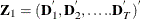 and
and  .
.
The matrix  contains the dummy variable structure for the two-way model.
For notational ease, let
![\[ {\Delta }_{N}= \mb{Z} ^{'}_{1} \mb{Z} _{1} \]](images/etsug_hppanel0107.png)
![\[ {\Delta }_{T}= \mb{Z} ^{'}_{2}\mb{Z} _{2} \]](images/etsug_hppanel0108.png)
![\[ \mb{A} = \mb{Z} ^{'}_{2}\mb{Z} _{1} \]](images/etsug_hppanel0109.png)
![\[ \bar{\mb{Z}}=\mb{Z} _{2}-\mb{Z} _{1} {\Delta }^{-1}_{N}\mb{A} ^{'} \]](images/etsug_hppanel0110.png)
![\[ \bar{\Delta }_{1}=\mb{I} _{M}-\mb{Z} _{1} {\Delta }^{-1}_{N}\mb{Z} ^{'}_{1} \]](images/etsug_hppanel0111.png)
![\[ \bar{\Delta }_{2}=\mb{I} _{M}-\mb{Z} _{2} {\Delta }^{-1}_{T}\mb{Z} ^{'}_{2} \]](images/etsug_hppanel0112.png)
![\[ \mb{Q} ={\Delta }_{T}-\mb{A} {\Delta }^{-1}_{N}\mb{A} ^{'} \]](images/etsug_hppanel0113.png)
![\[ \mb{P} =(\mb{I} _{M}- \mb{Z} _{1} {\Delta }^{-1}_{N}\mb{Z} ^{'}_{1}) - \bar{\mb{Z}}\mb{Q}^{-1}\bar{\mb{Z}}^{'} \]](images/etsug_hppanel0114.png)
PROC HPPANEL provides four methods to estimate the variance components. For more information, see the section Two-Way Random-Effects Model.
After the estimates of the variance components are calculated, you can proceed to the final estimation. If the panel is balanced, partial mean deviations are used as follows
![\[ \tilde{y}_\mi {it} = y_\mi {it}- \theta _{1} \bar{y}_\mi {i \cdot } - \theta _{2} \bar{y}_\mi {\cdot t} + \theta _{3} \bar{y}_\mi {\cdot \cdot } \]](images/etsug_hppanel0115.png)
![\[ \tilde{x}_\mi {it} = x_\mi {it}- \theta _{1} \bar{x}_\mi {i \cdot } - \theta _{2} \bar{x}_\mi {\cdot t} + \theta _{3} \bar{x}_\mi {\cdot \cdot } \]](images/etsug_hppanel0116.png)
The  estimates are obtained from
![\[ \theta _{1} = 1 - \frac{\sigma _{\epsilon }}{\sqrt {T\sigma _{\nu }^{2} + \sigma _{\epsilon }^{2}}} \]](images/etsug_hppanel0118.png)
![\[ \theta _{2} = 1 - \frac{\sigma _{\epsilon }}{\sqrt {N\sigma _{e}^{2} + \sigma _{\epsilon }^{2}}} \]](images/etsug_hppanel0119.png)
![\[ \theta _{3} = \theta _{1} + \theta _{2} + \frac{\sigma _{\epsilon }}{\sqrt {T\sigma _{\nu }^{2} + N\sigma _{e}^{2} + \sigma _{\epsilon }^{2}}}- 1 \]](images/etsug_hppanel0120.png)
With these partial deviations, PROC HPPANEL uses OLS on the transformed series (including an intercept if you want).
The case of an unbalanced panel is somewhat more complicated. Wansbeek and Kapteyn show that the inverse of  can be written as
![\[ \sigma _{\epsilon }^{2}\Omega ^{-1} = \mb{V}- \mb{V}\mb{Z}_2\tilde{\mb{P}}^{-1}\mb{Z}_2^{'}\mb{V} \]](images/etsug_hppanel0122.png)
with the following:
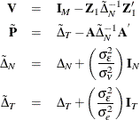
By using the inverse of the covariance matrix of the error, it becomes possible to complete GLS on the unbalanced panel.