The SEVERITY Procedure
- Overview
-
Getting Started

-
Syntax
-
Details
Predefined Distributions Censoring and Truncation Parameter Estimation Method Parameter Initialization Estimating Regression Effects Empirical Distribution Function Estimation Methods Statistics of Fit Defining a Distribution Model with the FCMP Procedure Predefined Utility Functions Custom Objective Functions Input Data Sets Output Data Sets Displayed Output ODS Graphics
-
Examples
Defining a Model for Gaussian Distribution Defining a Model for Gaussian Distribution with a Scale Parameter Defining a Model for Mixed-Tail Distributions Estimating Parameters Using Cramér-von Mises Estimator Fitting a Scaled Tweedie Model with Regressors Fitting Distributions to Interval-Censored Data
- References
Example 23.2 Defining a Model for Gaussian Distribution with a Scale Parameter
If you want to estimate the effects of regressors, then the model needs to be parameterized to have a scale parameter. While this might not be always possible, for the case of the Gaussian distribution it is possible by replacing the location parameter  with another parameter,
  , and defining the PDF (
 ) and the CDF (
 ) as follows:
 |
 |
|||
 |
 |
It can be verified that  is the scale parameter, because both of the following equalities are true:
|
 |
|||
|
 |
Note: The Gaussian distribution is not a commonly used severity distribution. It is used in this example primarily to illustrate the concept of parameterizing a distribution such that it has a scale parameter. Although the distribution has a support over the entire real line, you can fit the distribution with PROC SEVERITY only if the input sample contains nonnegative values.
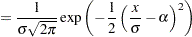
The following statements use the alternate parameterization to define a new model named NORMAL_S. The definition is stored in the Work.Sevexmpl library.
/*-------- Define Normal Distribution With Scale Parameter ----------*/
proc fcmp library=sashelp.svrtdist outlib=work.sevexmpl.models;
function normal_s_pdf(x, Sigma, Alpha);
/* Sigma : Scale & Standard Deviation */
/* Alpha : Scaled mean */
return ( exp(-(x/Sigma - Alpha)**2/2) /
(Sigma * sqrt(2*constant('PI'))) );
endsub;
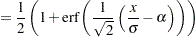
function normal_s_cdf(x, Sigma, Alpha);
/* Sigma : Scale & Standard Deviation */
/* Alpha : Scaled mean */
z = x/Sigma - Alpha;
return (0.5 + 0.5*erf(z/sqrt(2)));
endsub;
subroutine normal_s_parminit(dim, x[*], nx[*], F[*], Ftype, Sigma, Alpha);
outargs Sigma, Alpha;
array m[2] / nosymbols;
/* Compute estimates by using method of moments */
call svrtutil_rawmoments(dim, x, nx, 2, m);
Sigma = sqrt(m[2] - m[1]**2);
Alpha = m[1]/Sigma;
endsub;
subroutine normal_s_lowerbounds(Sigma, Alpha);
outargs Sigma, Alpha;
Alpha = .; /* Alpha has no lower bound */
Sigma = 0; /* Sigma > 0 */
endsub;
quit;
An important point to note is that the scale parameter Sigma is the first distribution parameter (after the 'x' argument) listed in the signatures of NORMAL_S_PDF and NORMAL_S_CDF functions. Sigma is also the first distribution parameter listed in the signatures of other subroutines. This is required by PROC SEVERITY, so that it can identify which is the scale parameter. When regressor variables are specified, PROC SEVERITY checks whether the first parameter of each candidate distribution is a scale parameter (or a log-transformed scale parameter if dist_SCALETRANSFORM subroutine is defined for the distribution with LOG as the transform). If it is not, then an appropriate message is written the SAS log and that distribution is not fitted.
Let the following DATA step statements simulate a sample from the normal distribution where the parameter is affected by the regressors as follows:
 |
The sample is simulated such that the regressor X2 is linearly dependent on regressors X1 and X3.
/*--- Simulate a Normal sample affected by Regressors ---*/
data testnorm_reg(keep=y x1-x5 Sigma);
   array x{*} x1-x5;
   array b{6} _TEMPORARY_ (1 0.5 . 0.75 -2 1);
   call streaminit(34567);
   label y='Normal Response Influenced by Regressors';

   do n = 1 to 100;
      /* simulate regressors */
      do i = 1 to dim(x);
         x(i) = rand('UNIFORM');
      end;
      /* make x2 linearly dependent on x1 and x3 */
      x(2) = x(1) + 5 * x(3);

      /* compute log of the scale parameter */
      logSigma = b(1);
      do i = 1 to dim(x);
         if (i ne 2) then
            logSigma = logSigma + b(i+1) * x(i);
      end;

      Sigma = exp(logSigma);
      y = rand('NORMAL', 25, Sigma);

      output;
   end;
run;
The following statements use PROC SEVERITY to fit the NORMAL_S distribution model along with some of the predefined distributions to the simulated sample:
/*--- Set the search path for functions defined with PROC FCMP ---*/
options cmplib=(work.sevexmpl);

/*-------- Fit models with PROC SEVERITY --------*/
proc severity data=testnorm_reg print=all plots=none;
   loss y;
   scalemodel x1-x5;
   dist Normal_s burr logn pareto weibull;
run;
The "Model Selection Table" in Output 23.2.1 indicates that all the models, except the Burr distribution model, have converged. Also, only three models, Normal_s, Burr, and Weibull, seem to have a good fit for the data. The table that compares all the fit statistics indicates that Normal_s model is the best according to the likelihood-based statistics; however, the Burr model is the best according to the EDF-based statistics.
| Input Data Set | |
|---|---|
| Name | WORK.TESTNORM_REG |
| Model Selection Table | |||
|---|---|---|---|
| Distribution | Converged | -2 Log Likelihood | Selected |
| Normal_s | Yes | 603.95786 | Yes |
| Burr | Maybe | 612.80861 | No |
| Logn | Yes | 749.20125 | No |
| Pareto | Yes | 841.07013 | No |
| Weibull | Yes | 612.77496 | No |
| All Fit Statistics Table | ||||||||||||||
|---|---|---|---|---|---|---|---|---|---|---|---|---|---|---|
| Distribution | -2 Log Likelihood |
AIC | AICC | BIC | KS | AD | CvM | |||||||
| Normal_s | 603.95786 | * | 615.95786 | * | 616.86108 | * | 631.58888 | * | 1.56822 | * | 4.25257 | 0.75658 | ||
| Burr | 612.80861 | 626.80861 | 628.02600 | 645.04480 | 1.59005 | 4.21979 | * | 0.71880 | * | |||||
| Logn | 749.20125 | 761.20125 | 762.10448 | 776.83227 | 2.89985 | 16.57630 | 3.13174 | |||||||
| Pareto | 841.07013 | 853.07013 | 853.97336 | 868.70115 | 4.83826 | 31.60773 | 6.84091 | |||||||
| Weibull | 612.77496 | 624.77496 | 625.67819 | 640.40598 | 1.59176 | 4.22441 | 0.71985 | |||||||
This prompts for further evaluation of why the model with Burr distribution has not converged. The initial values, convergence status, and the optimization summary for the Burr distribution are shown in Output 23.2.2. The initial values table indicates that the regressor X2 is redundant, which is expected. More importantly, the convergence status indicates that it requires more than 50 iterations. PROC SEVERITY enables you to change several settings of the optimizer by using the NLOPTIONS statement. In this case, you can increase the limit of 50 on the iterations, change the convergence criterion, or change the technique to something other than the default trust-region technique.
| Distribution Information | |
|---|---|
| Name | Burr |
| Description | Burr Distribution |
| Number of Distribution Parameters | 3 |
| Number of Regression Parameters | 4 |
| Initial Parameter Values and Bounds for Burr Distribution |
|||
|---|---|---|---|
| Parameter | Initial Value | Lower Bound | Upper Bound |
| Theta | 25.75198 | 1.05367E-8 | Infty |
| Alpha | 2.00000 | 1.05367E-8 | Infty |
| Gamma | 2.00000 | 1.05367E-8 | Infty |
| x1 | 0.07345 | -709.78271 | 709.78271 |
| x2 | Redundant | . | . |
| x3 | -0.14056 | -709.78271 | 709.78271 |
| x4 | 0.27064 | -709.78271 | 709.78271 |
| x5 | -0.23230 | -709.78271 | 709.78271 |
| Convergence Status for Burr Distribution |
|---|
| Needs more than 50 iterations. |
| Optimization Summary for Burr Distribution | |
|---|---|
| Optimization Technique | Trust Region |
| Number of Iterations | 50 |
| Number of Function Evaluations | 130 |
| Log Likelihood | -306.40430 |
The following PROC SEVERITY step uses the NLOPTIONS statement to change the convergence criterion and the limits on the iterations and function evaluations, exclude the lognormal and Pareto distributions that have been confirmed previously to fit the data poorly, and exclude the redundant regressor X2 from the model:
/*--- Refit and compare models with higher limit on iterations ---*/
proc severity data=testnorm_reg print=all plots=pp;
   loss y;
   scalemodel x1 x3-x5;
   dist Normal_s burr weibull;
   nloptions absfconv=2.0e-5 maxiter=100 maxfunc=500;
run;
The results shown in Output 23.2.3 indicate that the Burr distribution has now converged and that the Burr and Weibull distributions have an almost identical fit for the data. The NORMAL_S distribution is still the best distribution according to the likelihood-based criteria.
| Input Data Set | |
|---|---|
| Name | WORK.TESTNORM_REG |
| Model Selection Table | |||
|---|---|---|---|
| Distribution | Converged | -2 Log Likelihood | Selected |
| Normal_s | Yes | 603.95786 | Yes |
| Burr | Yes | 612.78605 | No |
| Weibull | Yes | 612.77496 | No |
| All Fit Statistics Table | ||||||||||||||
|---|---|---|---|---|---|---|---|---|---|---|---|---|---|---|
| Distribution | -2 Log Likelihood |
AIC | AICC | BIC | KS | AD | CvM | |||||||
| Normal_s | 603.95786 | * | 615.95786 | * | 616.86108 | * | 631.58888 | * | 1.56822 | * | 4.25257 | 0.75658 | ||
| Burr | 612.78605 | 626.78605 | 628.00344 | 645.02224 | 1.59154 | 4.22313 | * | 0.71959 | * | |||||
| Weibull | 612.77496 | 624.77496 | 625.67819 | 640.40598 | 1.59176 | 4.22441 | 0.71985 | |||||||
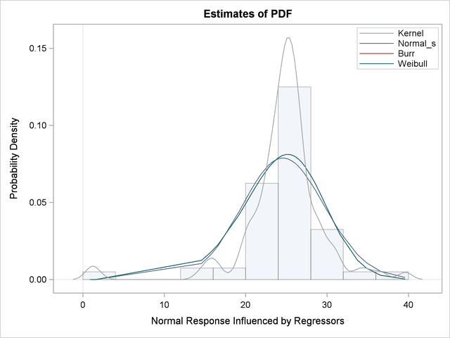
The comparison of the PDF estimates of all the candidates is shown in Output 23.2.4. Each plotted PDF estimate is an average computed over the  PDF estimates that are obtained with the scale parameter determined by each of the observations in the input data set. The PDF plot shows that the Burr and Weibull models result in almost identical estimates. All the estimates have a slight left skew with the mode closer to Y=25, which is the mean of the simulated sample.
The P-P plots for the Normal_s and Burr distributions are shown in Output 23.2.5. These plots show how the EDF estimates compare against the CDF estimates. Each plotted CDF estimate is an average computed over the CDF estimates that are obtained with the scale parameter determined by each of the observations in the input data set. Comparing the P-P plots of Normal_s and Burr distributions indicates that both fit the data almost similarly, but the Burr distribution fits the right tail slightly better, which explains why the EDF-based statistics prefer it over the Normal_s distribution.
|
![\includegraphics[width=3.15in]{png/sevex02o5g.png}](images/etsug_severity0664.png) |
![\includegraphics[width=3.15in]{png/sevex02o5g1.png}](images/etsug_severity0665.png) |