The SEVERITY Procedure

Likelihood Function

Let and denote the PDF and CDF, respectively, evaluated at for a set of parameter values . Let denote the random response variable, and let denote its value recorded in an observation in the input data set. Let and denote the random variables for the left-truncation and right-truncation threshold, respectively, and let and denote their values for an observation, respectively. If there is no left-truncation, then , where is the smallest value in the support of the distribution; so . If there is no right-truncation, then , where is the largest value in the support of the distribution; so . Let and denote the random variables for the left-censoring and right-censoring limit, respectively, and let and denote their values for an observation, respectively. If there is no left-censoring, then , so . If there is no right-censoring, then , so .

The set of input observations can be categorized into the following four subsets within each BY group:

• is the set of uncensored and untruncated observations. The likelihood of an observation in is

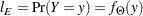
• is the set of uncensored observations that are truncated. The likelihood of an observation in is

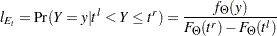
• is the set of censored observations that are not truncated. The likelihood of an observation is

• is the set of censored observations that are truncated. The likelihood of an observation is

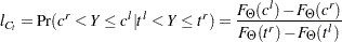
Note that 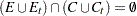. Also, the sets and are empty when no truncation is specified, and the sets and are empty when no censoring is specified.

Given this, the likelihood of the data is as follows:

The maximum likelihood procedure used by PROC SEVERITY finds an optimal set of parameter values that maximizes subject to the boundary constraints on parameter values. For a distribution dist, such boundary constraints can be specified by using the dist_LOWERBOUNDS and dist_UPPERBOUNDS subroutines. See the section Defining a Distribution Model with the FCMP Procedure for details. Some aspects of the optimization process can be controlled by using the NLOPTIONS statement.

Probability of Observability and Likelihood

If probability of observability is specified for the left-truncation, then PROC SEVERITY uses a modified likelihood function for each truncated observation. If the probability of observability is , then for each left-truncated observation with truncation threshold , there exist observations with a response variable value less than or equal to . Each such observation has a probability of 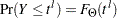. The right-truncation and censoring information does not apply to these added observations. Thus, following the notation of the section Likelihood Function, the likelihood of the data is as follows:

Note that the likelihood of the observations that are not left-truncated (observations in sets and , and observations in sets and for which ) is not affected.

If you have specified a custom objective function, then PROC SEVERITY accounts for the probability of observability only while computing the empirical distribution function estimate. The parameter estimates are affected only by your custom objective function.

Estimating Covariance and Standard Errors

PROC SEVERITY computes an estimate of the covariance matrix of the parameters by using the asymptotic theory of the maximum likelihood estimators (MLE). If denotes the number of observations used for estimating a parameter vector , then the theory states that as , the distribution of , the estimate of , converges to a normal distribution with mean and covariance such that , where 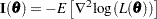is the information matrix for the likelihood of the data, . The covariance estimate is obtained by using the inverse of the information matrix.

In particular, if 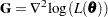denotes the Hessian matrix of the log likelihood, then the covariance estimate is computed as

where is a denominator determined by the VARDEF= option. If VARDEF=N, then , which yields the asymptotic covariance estimate. If VARDEF=DF, then , where is number of parameters (the model’s degrees of freedom). The VARDEF=DF option is the default, because it attempts to correct the potential bias introduced by the finite sample.

The standard error of the parameter is computed as the square root of the th diagonal element of the estimated covariance matrix; that is, .

If you have specified a custom objective function, then the covariance matrix of the parameters is still computed by inverting the information matrix, except that the Hessian matrix is computed as , where denotes your custom objective function.

Covariance and standard error estimates might not be available if the Hessian matrix is found to be singular at the end of the optimization process. This can especially happen if the optimization process stops without converging.