The SEVERITY Procedure
- Overview
-
Getting Started

-
Syntax
-
Details
Predefined Distributions Censoring and Truncation Parameter Estimation Method Parameter Initialization Estimating Regression Effects Empirical Distribution Function Estimation Methods Statistics of Fit Defining a Distribution Model with the FCMP Procedure Predefined Utility Functions Custom Objective Functions Input Data Sets Output Data Sets Displayed Output ODS Graphics
-
Examples
Defining a Model for Gaussian Distribution Defining a Model for Gaussian Distribution with a Scale Parameter Defining a Model for Mixed-Tail Distributions Estimating Parameters Using Cramér-von Mises Estimator Fitting a Scaled Tweedie Model with Regressors Fitting Distributions to Interval-Censored Data
- References
| Estimating Regression Effects |
The SEVERITY procedure enables you to estimate the effects of regressor (exogenous) variables while fitting a distribution if the distribution has a scale parameter or a log-transformed scale parameter.
Let  (
( ) denote the
  regressor variables. Let
  denote the regression parameter that corresponds to the regressor . If regression effects are not specified, then the model for the response variable
  is of the form
 |
where  is the distribution of with parameters
  . This model is typically referred to as the error model. The regression effects are modeled by extending the error model to the following form:
 |
Under this model, the distribution of is valid and belongs to the same parametric family as if and only if has a scale parameter. Let  denote the scale parameter and
  denote the set of nonscale distribution parameters of . Then the model can be rewritten as
 |
such that is affected by the regressors as
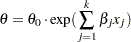 |
where  is the base value of the scale parameter. Thus, the regression model consists of the following parameters: , , and
  .
.
Given this form of the model, distributions without a scale parameter cannot be considered when regression effects are to be modeled. If a distribution does not have a direct scale parameter, then PROC SEVERITY accepts it only if it has a log-transformed scale parameter — that is, if it has a parameter  .
.
Parameter Initialization for Regression Models
The regression parameters are initialized either by using the values you specify or by the default method.
-
If you provide initial values for the regression parameters, then you must provide valid, nonmissing initial values for
and parameters for all  .
. You can specify the initial value for
using either the INEST= data set or the INIT= option in the DIST statement. If the distribution has a direct scale parameter (no transformation), then the initial value for the first parameter of the distribution is used as an initial value for . If the distribution has a log-transformed scale parameter, then the initial value for the first parameter of the distribution is used as an initial value for  .
. You can use only the INEST= data set to specify the initial values for
. The INEST= data set must contain nonmissing initial values for all the regressors specified in the SCALEMODEL statement. The only missing value allowed is the special missing value .R, which indicates that the regressor is linearly dependent on other regressors. If you specify .R for a regressor for one distribution in a BY group, you must specify it so for all the distributions in that BY group. -
If you do not specify valid initial values for
or parameters for all , then PROC SEVERITY initializes those parameters using the following method: Let a random variable
be distributed as  , where is the scale parameter. By definition of the scale parameter, a random variable
  is distributed as
  such that
 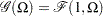 . Given a random error term
  that is generated from a distribution , a value
  from the distribution of can be generated as
Taking the logarithm of both sides and using the relationship of
with the regressors yields: 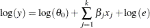
PROC SEVERITY makes use of the preceding relationship to initialize parameters of a regression model with distribution dist as follows:
-
The following linear regression problem is solved to obtain initial estimates of
 and :
and : 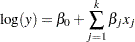
The estimates of
in the solution of this regression problem are used to initialize the respective regression parameters of the model. The estimate of is later used to initialize the value of . The results of this regression are also used to detect whether any regressors are linearly dependent on the other regressors. If any such regressors are found, then a warning is written to the SAS log and the corresponding regressor is eliminated from further analysis. The estimates for linearly dependent regressors are denoted by a special missing value of .R in the OUTEST= data set and in any displayed output.
-
Let
 denote the initial value of the scale parameter.
 If the distribution model of dist does not contain the dist_PARMINIT subroutine, then
and all the nonscale distribution parameters are initialized to the default value of 0.001. However, it is strongly recommended that each distribution’s model contain the dist_PARMINIT subroutine. See the section Defining a Distribution Model with the FCMP Procedure for more details. If that subroutine is defined, then
is initialized as follows: Each input value
 of the response variable is transformed to its scale-normalized version
  as
as 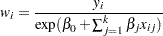
where
 denotes the value of th regressor in the
  th input observation. These values are used to compute the input arguments for the dist_PARMINIT subroutine. The values that are computed by the subroutine for nonscale parameters are used as their respective initial values. If the distribution has an untransformed scale parameter, then is set to the value of the scale parameter that is computed by the subroutine. If the distribution has a log-transformed scale parameter
  , then is computed as
  , where
  is the value of computed by the subroutine.
 -
The value of
is initialized as 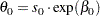
-
Reporting Estimates of Regression Parameters
When you request estimates to be written to the output (either ODS displayed output or in the OUTEST= data set), the estimate of the base value of the first distribution parameter is reported. If the first parameter is the log-transformed scale parameter, then the estimate of is reported; otherwise, the estimate of is reported. The transform of the first parameter of a distribution dist is controlled by the dist_SCALETRANSFORM function that is defined for it.
CDF and PDF Estimates with Regression Effects
When regression effects are estimated, the estimate of the scale parameter depends on the values of the regressors and estimates of the regression parameters. This results in a potentially different distribution for each observation. In order to make estimates of the cumulative distribution function (CDF) and probability density function (PDF) comparable across distributions and comparable to the empirical distribution function (EDF), PROC SEVERITY reports the CDF and PDF estimates from a mixture distribution. This mixture distribution is an equally weighted mixture of  distributions, where is the number of observations used for estimation. Each component of the mixture differs only in the value of the scale parameter.
In particular, let  and
and  denote the PDF and CDF, respectively, of the component distribution due to observation , where denotes the value of the response variable,
  denotes the estimate of the scale parameter due to observation , and
  denotes the set of estimates of all other parameters of the distribution. The value of
  is computed as
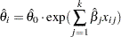 |
where  is an estimate of the base value of the scale parameter,
  are the estimates of regression coefficients, and is the value of regressor in observation . Then, the PDF and CDF estimates,
  and
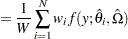
and  , respectively, of the mixture distribution at are computed as follows:
 |
 |
|||
 |
 |
where denotes the weight of observation and  is the total weight (
 ). If the WEIGHT statement is specified, then the weight is equal to the value of the specified weight variable; otherwise, the weight is equal to 1.
The CDF estimates reported in OUTCDF= data set and plotted in CDF plots are the values. The PDF estimates plotted in PDF plots are the values.
If truncation is specified, then the conditional CDF estimates are computed by using the value along with the minimum and maximum truncation limits as described in the section Truncation and Conditional CDF Estimates.