The SEVERITY Procedure
- Overview
-
Getting Started

-
Syntax
-
Details
Predefined Distributions Censoring and Truncation Parameter Estimation Method Parameter Initialization Estimating Regression Effects Empirical Distribution Function Estimation Methods Statistics of Fit Defining a Distribution Model with the FCMP Procedure Predefined Utility Functions Custom Objective Functions Input Data Sets Output Data Sets Displayed Output ODS Graphics
-
Examples
Defining a Model for Gaussian Distribution Defining a Model for Gaussian Distribution with a Scale Parameter Defining a Model for Mixed-Tail Distributions Estimating Parameters Using Cramér-von Mises Estimator Fitting a Scaled Tweedie Model with Regressors Fitting Distributions to Interval-Censored Data
- References
Example 23.1 Defining a Model for Gaussian Distribution
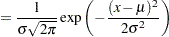
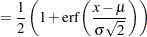
Suppose you want to fit a distribution model other than one of the predefined ones available to you. Suppose you want to define a model for the Gaussian distribution with the following typical parameterization of the PDF ( ) and CDF (
 ):
):
 |
 |
|||
 |
 |
For PROC SEVERITY, a distribution model consists of a set of functions and subroutines that are defined with the FCMP procedure. Each function and subroutine should be written following certain rules. The details are provided in the section Defining a Distribution Model with the FCMP Procedure.
Note: The Gaussian distribution is not a commonly used severity distribution. It is used in this example primarily to illustrate the process of defining your own distribution models. Although the distribution has a support over the entire real line, you can fit the distribution with PROC SEVERITY only if the input sample contains nonnegative values.
The following SAS statements define a distribution model named NORMAL for the Gaussian distribution. The OUTLIB= option in the PROC FCMP statement stores the compiled versions of the functions and subroutines in the 'models' package of the Work.Sevexmpl library. The LIBRARY= option in the PROC FCMP statement enables this PROC FCMP step to use the SVRTUTIL_RAWMOMENTS utility subroutine that is available in the Sashelp.Svrtdist library. The subroutine is described in the section Predefined Utility Functions.
/*-------- Define Normal Distribution with PROC FCMP  ----------*/
proc fcmp library=sashelp.svrtdist outlib=work.sevexmpl.models;
   function normal_pdf(x,Mu,Sigma);
      /* Mu   : Location */
      /* Sigma : Standard Deviation */
      return ( exp(-(x-Mu)**2/(2 * Sigma**2)) /
             (Sigma * sqrt(2*constant('PI'))) );
   endsub;

   function normal_cdf(x,Mu,Sigma);
      /* Mu   : Location */
      /* Sigma : Standard Deviation */
      z = (x-Mu)/Sigma;
      return (0.5 + 0.5*erf(z/sqrt(2)));
   endsub;

   subroutine normal_parminit(dim, x[*], nx[*], F[*], Ftype, Mu, Sigma);
      outargs Mu, Sigma;
      array m[2] / nosymbols;

      /* Compute estimates by using method of moments */
      call svrtutil_rawmoments(dim, x, nx, 2, m);
      Mu   = m[1];
      Sigma = sqrt(m[2] - m[1]**2);
   endsub;

   subroutine normal_lowerbounds(Mu, Sigma);
      outargs Mu, Sigma;
      Mu = .;   /* Mu has no lower bound */
      Sigma = 0; /* Sigma > 0 */
   endsub;
quit;
The statements define the two functions required of any distribution model (NORMAL_PDF and NORMAL_CDF) and two optional subroutines (NORMAL_PARMINIT and NORMAL_LOWERBOUNDS). The name of each function or subroutine must follow a specific structure. It should start with the model’s short or identifying name, which is 'NORMAL' in this case, followed by an underscore '_', followed by a keyword suffix such as 'PDF'. Each function or subroutine has a specific purpose. The details of all the functions and subroutines that you can define for a distribution model are provided in the section Defining a Distribution Model with the FCMP Procedure. Following is the description of each function and subroutine defined in this example:
The PDF and CDF suffixes define functions that return the probability density function and cumulative distribution function values, respectively, given the values of the random variable and the distribution parameters.
-
The PARMINIT suffix defines a subroutine that returns the initial values for the parameters by using the sample data or the empirical distribution function (EDF) estimate computed from it. In this example, the parameters are initialized by using the method of moments. Hence, you do not need to use the EDF estimates, which are available in the F array. The first two raw moments of the Gaussian distribution are as follows:
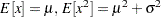
Given the sample estimates,
 and
and  , of these two raw moments, you can solve the equations
  and
and  to get the following estimates for the parameters:
  and
and  . The NORMAL_PARMINIT subroutine implements this solution. It uses the SVRTUTIL_RAWMOMENTS utility subroutine to compute the first two raw moments.
 The LOWERBOUNDS suffix defines a subroutine that returns the lower bounds on the parameters. PROC SEVERITY assumes a default lower bound of 0 for all the parameters when a LOWERBOUNDS subroutine is not defined. For the parameter
 (Mu), there is no lower bound, so you need to define the NORMAL_LOWERBOUNDS subroutine. It is recommended that you assign bounds for all the parameters when you define the LOWERBOUNDS subroutine or its counterpart, the UPPERBOUNDS subroutine. Any unassigned value is returned as a missing value, which is interpreted by PROC SEVERITY to mean that the parameter is unbounded, and that might not be what you want.
You can now use this distribution model with PROC SEVERITY. Let the following DATA step statements simulate a normal sample with  and
and  .
.
/*-------- Simulate a Normal sample ----------*/
data testnorm(keep=y);
   call streaminit(12345);
   do i=1 to 100;
      y = rand('NORMAL', 10, 2.5);
      output;
   end;
run;
Prior to using your distribution with PROC SEVERITY, you must communicate the location of the library that contains the definition of the distribution and the locations of libraries that contain any functions and subroutines used by your distribution model. The following OPTIONS statement sets the CMPLIB= system option to include the FCMP library Work.Sevexmpl in the search path used by PROC SEVERITY to find FCMP functions and subroutines.
/*--- Set the search path for functions defined with PROC FCMP ---*/
options cmplib=(work.sevexmpl);
Now, you are ready to fit the NORMAL distribution model with PROC SEVERITY. The following statements fit the model to the values of Y in the Work.Testnorm data set:
/*--- Fit models with PROC SEVERITY ---*/
proc severity data=testnorm print=all;
   loss y;
   dist Normal;
run;
The DIST statement specifies the identifying name of the distribution model, which is 'NORMAL'. Neither is the INEST= option specified in the PROC SEVERITY statement nor is the INIT= option specified in the DIST statement. So, PROC SEVERITY initializes the parameters by invoking the NORMAL_PARMINIT subroutine.
Some of the results prepared by the preceding PROC SEVERITY step are shown in Output 23.1.1 and Output 23.1.2. The descriptive statistics of variable Y and the "Model Selection Table", which includes just the normal distribution, are shown in Output 23.1.1.
| Input Data Set | |
|---|---|
| Name | WORK.TESTNORM |
| Descriptive Statistics for Variable y | |
|---|---|
| Number of Observations | 100 |
| Number of Observations Used for Estimation | 100 |
| Minimum | 3.88249 |
| Maximum | 16.00864 |
| Mean | 10.02059 |
| Standard Deviation | 2.37730 |
| Model Selection Table | |||
|---|---|---|---|
| Distribution | Converged | -2 Log Likelihood | Selected |
| Normal | Yes | 455.97541 | Yes |
The initial values for the parameters, the optimization summary, and the final parameter estimates are shown in Output 23.1.2. No iterations are required to arrive at the final parameter estimates, which are identical to the initial values. This confirms the fact that the maximum likelihood estimates for the Gaussian distribution are identical to the estimates obtained by the method of moments that was used to initialize the parameters in the NORMAL_PARMINIT subroutine.
| Distribution Information | |
|---|---|
| Name | Normal |
| Number of Distribution Parameters | 2 |
| Initial Parameter Values and Bounds for Normal Distribution |
|||
|---|---|---|---|
| Parameter | Initial Value | Lower Bound | Upper Bound |
| Mu | 10.02059 | -Infty | Infty |
| Sigma | 2.36538 | 1.05367E-8 | Infty |
| Optimization Summary for Normal Distribution | |
|---|---|
| Optimization Technique | Trust Region |
| Number of Iterations | 0 |
| Number of Function Evaluations | 2 |
| Log Likelihood | -227.98770 |
| Parameter Estimates for Normal Distribution | ||||
|---|---|---|---|---|
| Parameter | Estimate | Standard Error |
t Value | Approx Pr > |t| |
| Mu | 10.02059 | 0.23894 | 41.94 | <.0001 |
| Sigma | 2.36538 | 0.16896 | 14.00 | <.0001 |
The NORMAL distribution defined and illustrated here has no scale parameter, because all the following inequalities are true:
|
 |
|||
 |
 |
|||
|
 |
|||
|
 |
This implies that you cannot estimate the effect of regressors on a model for the response variable based on this distribution.