The SEVERITY Procedure

Notation

Let there be a set of observations, each containing a quintuplet of values 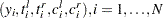, where is the value of the response variable, is the value of the left-truncation threshold, is the value of the right-truncation threshold, is the value of the left-censoring limit, and is the value of the right-censoring limit.

If an observation is not left-truncated, then , where is the smallest value in the support of the distribution; so . If an observation is not right-truncated, then , where is the largest value in the support of the distribution; so . If an observation is not left-censored, then ; so . If an observation is not right-censored, then ; so .

An indicator function takes a value of 1 or 0 if the expression is true or false, respectively.

EDF Estimation for No Censoring or Single Type of Censoring

These methods are described in detail assuming that all observations either uncensored or right-censored; that is, each observation is of the form .

If all observations are either uncensored or left-censored, then each observation is of the form . It is converted to an observation 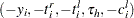; that is, the signs of all the response variable values are reversed, the new left-truncation threshold is equal to the negative of the original right-truncation threshold, the new right-truncation threshold is equal to the negative of the original left-truncation threshold, and the negative of the original left-censoring limit becomes the new right-censoring limit. With this transformation, each observation is either uncensored or right-censored. The methods described for handling uncensored or right-censored data are now applicable. After the EDF estimates are computed, the observations are transformed back to the original form and EDF estimates are adjusted such 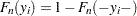, where denotes the EDF estimate of the value slightly less than the transformed value .

A set of uncensored or right-censored observations can be converted to a set of observations of the form , where is the indicator of right-censoring. indicates a right-censored observation, in which case is assumed to record the right-censoring limit . indicates an uncensored observation, and records the exact observed value. In other words, and .

Given this notation, the EDF is estimated as

where denotes the th order statistic of the set and is the estimate computed at that value. The definition of depends on the estimation method. You can specify a particular method or let PROC SEVERITY choose an appropriate method by using the EMPIRICALCDF= option in the PROC SEVERITY statement. Each method computes as follows:

STANDARD

This method is the standard way of computing EDF. The EDF estimate at observation is computed as follows:

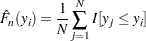
This method ignores any censoring and truncation information, even if it is specified. When no censoring or truncation information is specified, this is the default method chosen.

KAPLANMEIER

The Kaplan-Meier (KM) estimator, also known as the product-limit estimator, was first introduced by Kaplan and Meier (1958) for censored data. Lynden-Bell (1971) derived a similar estimator for left-truncated data. PROC SEVERITY uses the definition that combines both censoring and truncation information (Klein and Moeschberger 1997, Lai and Ying 1991).

The EDF estimate at observation is computed as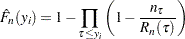

where and are defined as follows:

• , which is the number of uncensored observations () for which the response variable value is equal to and is observable according to the right-truncation threshold of that observation ().

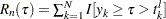• , which is the size (cardinality) of the risk set at . The term risk set has its origins in survival analysis; it contains the events that are at risk of failure at a given time, . In other words, it contains the events that have survived up to time and might fail at or after . For PROC SEVERITY, time is equivalent to the magnitude of the event and failure is equivalent to an uncensored and observable event, where observable means it satisfies the truncation thresholds.

If you do not explicitly specify a method of computing EDF, then this is the default method used if you specify either right-censoring or left-censoring, but not both. This is also the default method when you specify truncation without any censoring.

MODIFIEDKM

The product-limit estimator used by the KAPLANMEIER method does not work well if the risk set size becomes very small. For right-censored data, the size can become small towards the right tail. For left-truncated data, the size can become small at the left tail and can remain so for the entire range of data. This was demonstrated by Lai and Ying (1991). They proposed a modification to the estimator that ignores the effects due to small risk set sizes.

The EDF estimate at observation is computed as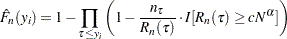

where the definitions of and are identical to those used for the KAPLANMEIER method described previously.

You can specify the values of and by using the C= and ALPHA= options. If you do not specify a value for , the default value used is . If you do not specify a value for , the default value used is .

As an alternative, you can also specify an absolute lower bound, say , on the risk set size by using the RSLB= option, in which case is replaced by in the definition.

EDF Estimation for Right-Censored and Left-Censored Data

If the response variable is subject to both left-censoring and right-censoring effects, then the SEVERITY procedure uses a method proposed by Turnbull (1976) to compute the nonparametric estimates of the cumulative distribution function. The original Turnbull’s method is modified using the suggestions made by Frydman (1994) when truncation effects are present.

Let the input data consist of observations in the form of quintuplets of values with notation described in the section Notation. For each observation, let be the censoring interval; that is, the response variable value is known to lie in the interval , but the exact value is not known. If an observation is uncensored, then for any arbitrarily small value of . If an observation is censored, then the value is ignored. Similarly, for each observation, let be the truncation interval; that is, the observation is drawn from a truncated (conditional) distribution .

Two sets, and , are formed using and as follows:

The sets and represent the left endpoints and right endpoints, respectively. A set of disjoint intervals , is formed such that and and and . The value of is dependent on the nature of censoring and truncation intervals in the input data. Turnbull (1976) showed that the maximum likelihood estimate (MLE) of the EDF can increase only inside intervals . In other words, the MLE estimate is constant in the interval . The likelihood is independent of the behavior of inside any of the intervals . Let denote the increase in inside an interval . Then, the EDF estimate is as follows:

PROC SEVERITY reports the estimates at points and and reports at point , where denotes the limiting estimate at a point that is infinitesimally larger than when approaching from values larger than and where denotes the limiting estimate at a point that is infinitesimally smaller than when approaching from values smaller than .

PROC SEVERITY uses the expectation-maximization (EM) algorithm proposed by Turnbull (1976), who referred to the algorithm as the self-consistency algorithm. By default, the algorithm runs until one of the following criteria is met:

• Relative-error criterion: The maximum relative error between the two consecutive estimates of falls below a threshold . If indicates an index of the current iteration, then this can be formally stated as

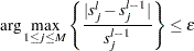
  You can control the value of by specifying the EPS= suboption of the EDF=TURNBULL option in the PROC SEVERITY statement. The default value is 1.0E–8.

• Maximum-iteration criterion: The number of iterations exceeds an upper limit specified by the MAXITER= suboption of the EDF=TURNBULL option in the PROC SEVERITY statement. The default number of maximum iterations is .

The self-consistent estimates obtained in this manner might not be maximum likelihood estimates. Gentleman and Geyer (1994) suggested the use of the Kuhn-Tucker conditions for the maximum likelihood problem to ensure that the estimates are MLE. If you specify the ENSUREMLE suboption of the EDF=TURNBULL option in the PROC SEVERITY statement, then PROC SEVERITY computes the Kuhn-Tucker conditions at the end of each iteration to determine whether the estimates {} are MLE. If no truncation effects are specified, then the Kuhn-Tucker conditions derived by Gentleman and Geyer (1994) are used. If truncation effects are specified, then PROC SEVERITY uses modified Kuhn-Tucker conditions that account for the truncation effects. An integral part of checking the conditions is to determine whether an estimate is zero or whether an estimate of the Lagrange multiplier or the reduced gradient associated with the estimate is zero. PROC SEVERITY declares these values to be zero if they are less than or equal to a threshold . You can control the value of by specifying the ZEROPROB= suboption of the EDF=TURNBULL option in the PROC SEVERITY statement. The default value is 1.0E–8. The algorithm continues until the Kuhn-Tucker conditions are satisfied or the number of iterations exceeds the upper limit. The relative-error criterion stated previously is not used when the ENSUREMLE option is specified.

EDF Estimates and Truncation

If truncation is specified, then the estimate computed by any method other than the STANDARD method is a conditional estimate. In other words, , where and denote the (unknown) distribution functions of the left-truncation threshold variable and the right-truncation threshold variable , respectively, denotes the smallest left-truncation threshold with a nonzero cumulative probability, and denotes the largest right-truncation threshold with a nonzero cumulative probability. Formally, and . For computational purposes, PROC SEVERITY estimates and by and , respectively, defined as

These estimates are used to compute conditional estimates of the CDF as described in the section Truncation and Conditional CDF Estimates.

If left-truncation is specified with the probability of observability , then PROC SEVERITY uses the additional information provided by to compute an estimate of the EDF that is not conditional on the left-truncation information. In particular, for each left-truncated observation with response variable value and truncation threshold , an observation is added with weight and . Each added observation is assumed to be uncensored and untruncated. Weight on each original observation is assumed to be 1; that is, . Then, the specified EDF method is used by assuming no left-truncation. The EDF estimate that is obtained using this method is not conditional on the left-truncation information. For the KAPLANMEIER and MODIFIEDKM methods with uncensored or right-censored data, definitions of and are modified to account for the weights on the observations. If denotes the total number of observations including the added observations, then is defined as , and is defined as 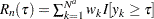. In the definition of , the left-truncation information is not used, because it was used along with to add the observations. If the original data are a combination of left- and right-censored data, then Turnbull’s method is applied to the appended set that contains no left-truncated observations.

Supplying EDF Estimates to Functions and Subroutines

The parameter initialization subroutines in distribution models and some predefined utility functions require EDF estimates. See the sections Defining a Distribution Model with the FCMP Procedure and Predefined Utility Functions for details.

PROC SEVERITY supplies the EDF estimates to these subroutines and functions by using two arrays, x and F, the dimension of each array, and a type of the EDF estimates. The type identifies how the EDF estimates are computed and stored. They are as follows:

Type 1

specifies that EDF estimates are computed using the STANDARD method; that is, the data used for estimation are neither censored nor truncated.

Type 2

specifies that EDF estimates are computed using either the KAPLANMEIER or the MODIFIEDKM method; that is, the data used for estimation are subject to truncation and one type of censoring (left or right, but not both).

Type 3

specifies that EDF estimates are computed using the TURNBULL method; that is, the data used for estimation are subject to both left- and right-censoring. The data might or might not be truncated.

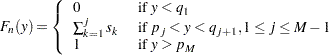
For Types 1 and 2, the EDF estimates are stored in arrays x and F of dimension N such that the following holds:

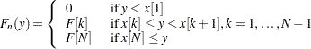where denotes th element of the array ([1] denotes the first element of the array).

For Type 3, the EDF estimates are stored in arrays x and F of dimension N such that the following holds:

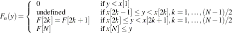Although the behavior of EDF is theoretically undefined for the interval , for computational purposes, all predefined functions and subroutines assume that the EDF increases linearly from to in that interval 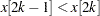if . If , which can happen when the EDF is estimated from a combination of uncensored and interval-censored data, the predefined functions and subroutines assume that .